Examples#
The examples have two jobs: a short Course teaches the framework itself, then Tours show what can be built on top of it. Every page is executable and uses the same public interfaces documented in the API reference.
Course#
Read the four Framework lessons in order. They are the shortest path from a shipped sequence to one of your own:
Getting started — run a shipped
torchsim.model.Simulator, inspect its sequence description, differentiate the signal, and see where execution happens.Expanded physics — turn on off-resonance, transmit variation, diffusion, flow, exchange and magnetization transfer without changing the sequence abstraction.
Writing a simulator — the extension point of the framework: subclass
torchsim.model.Simulator, choose the command handlers that interpret an incoming Pulseq/MRD event stream, and implementtorchsim.model.Simulator.layout()for offline construction.Custom operator — package a preparation or readout as an operator while leaving the state-machine kernels untouched.
A simulator is deliberately the common object in both directions. Offline,
layout() builds the sequence description. During acquisition,
Simulator.from_description() takes the description decoded from the
scanner’s MRD stream and replays the RF/ADC commands through the simulator’s
handlers. The physics, differentiation, execution policy, estimators and
reconstruction code therefore see the same object in either case.
Tours#
The remaining sections are standalone applications. They assume the Course, but not one another.
Parameter inference compares dictionary matching, lookup tables, nonlinear least squares and PERK on the same mapping problem.
Sequence optimization differentiates through the simulator to design echo trains, quantitative schedules and RF pulses.
Model-based imaging places the simulator inside the forward model, through a linear subspace or nonlinear inversion.
Miscellaneous contains complete pipelines that do not belong to the linear course.
Framework#
How to use TorchSim, and how to extend it.
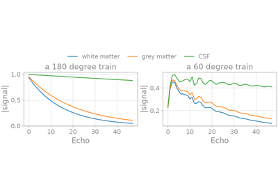
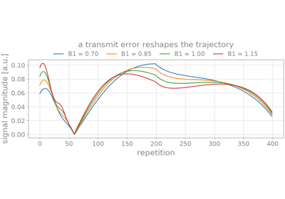
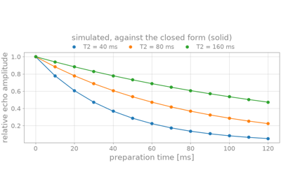
The first notebook covers basic usage: simulating a signal, taking its derivatives, tuning the run, and reading a sequence back from the description a scanner streams. The second covers the physics a simulator can carry beyond T1 and T2.
The last two are for sequences TorchSim does not ship. A signal model of your own is two pieces – a physics saying what each kind of event does, and a simulator saying what order they are played in. An operator of your own – a preparation, a readout – is a Python function that returns events.
None of it requires touching a kernel.
Parameter inference#
Estimating tissue properties from a measured volume.
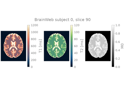
Every estimator is made from the simulator it inverts and fitted over the same statement of the problem – what is unknown, over what range, at what noise level – and they differ only in how they fill it in. These examples change only that: dictionary matching over a parameter grid, compressed and clustered; interpolation along a curve where there is a single unknown; a nonlinear fit of the model itself; and a kernel regression that never builds a grid at all.
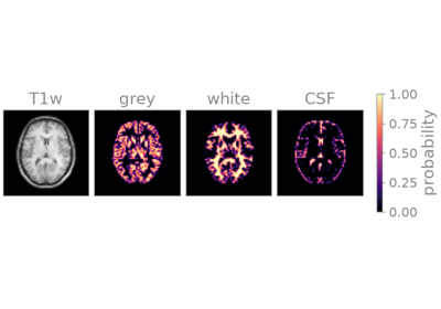
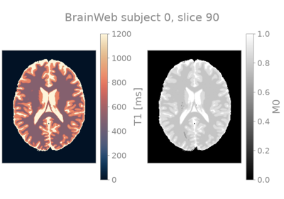
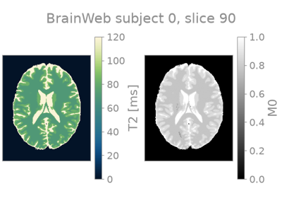
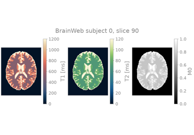
Every one of them maps the same BrainWeb slice, so the answer is known everywhere – mixtures of tissues included – and reports what it cost in time and in memory alongside what it got wrong.
Sequence optimization#
Choosing a sequence’s parameters rather than simulating the ones you were given.
A design problem is three pieces: a simulator with the tissue it is designed
for already fixed on it; a cost, which is a plain function of what that
simulator records; and a SequenceDesign, which holds the
parameters inside the limits the scanner will play and runs the loop.
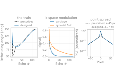
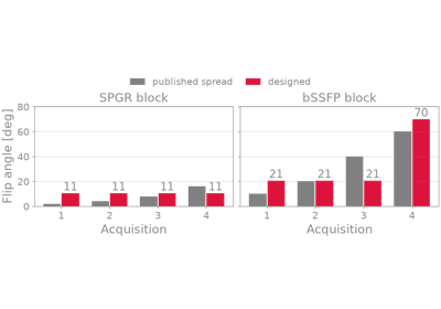
Only the cost changes between the first two examples here. One asks for a picture – sharp where sharpness is decided, with contrast where contrast is decided – and the other asks for precision, choosing flip angles so that T1 and T2 are estimated as tightly as the scan time allows.
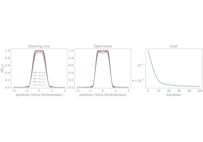
The third designs no protocol parameter at all but the samples of an RF pulse, through a Bloch simulation of the slice it excites, so that the excitation holds where the transmit field does not.
Model-based imaging#
Reconstructing parameter maps from k-space without forming the contrast images in between.
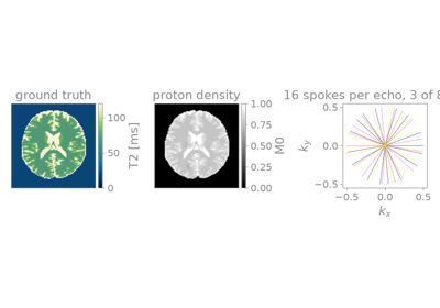
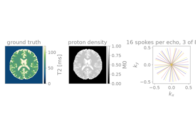
A quantitative scan is usually reconstructed twice: once to make one image per contrast, and again – voxel by voxel – to turn those images into maps. The first step has no idea what the second one is for. Writing the signal model into the forward operator removes the intermediate step, and the echoes then constrain one another instead of being recovered separately.
There are two ways to do it. A linear subspace writes the signal in the low-rank basis the train spans and reconstructs the coefficients, which stays linear and so has no local minima and no starting guess. Nonlinear inversion keeps the model itself inside the operator and solves for the maps directly, which costs more and is what a signal with no small basis needs.
Miscellaneous#
Everything that is a pipeline rather than a demonstration of a call.