5. Testing on the virtual scanner

This lesson is optional: it extends the course rather than completing it. The virtual scanner stands in for the scanner and nothing else, so a sequence and a reconstruction plugin can be tested before a scanner is involved. Its Fourier engine acquires a phantom’s tissue under every RF pulse, gradient and receiver phase the cache plays, with relaxation, so a scan shows the contrast and the artefacts of the sequence as well as its encoding. The conversion itself is checked by comparing the gradients a sequence asks for with those its cache plays. The model is described in The virtual scanner.

Learning objectives

• Acquire a phantom’s tissue with simulate(), and compare the contrast of the images with the closed-form steady state of the sequence.

• Check a cache against the sequence it was converted from with validate().

The previous lesson reconstructed a series with a plugin of its own.

A sequence with T1 contrast

The design is the RF-spoiled 2D gradient echo at a 20 ms TR and a 30° flip angle, converted into its cache twice: without dummy scans, and with 100, which play for 2 s before the first readout. The phantom holds two ellipses of equal proton density and T2, with a T1 of 300 ms on the left and 1500 ms on the right.

import tempfile
from pathlib import Path

import numpy as np
import pypulseqpp as pp
from pypulseqpp.sequences.sequence.gre2D_sequence import gre2d

from pulserver import ir, virtual
from pulserver.proxy import SequenceTable

TR, FLIP, T1 = 0.02, np.radians(30.0), (0.3, 1.5)

system = pp.Opts(max_grad=40, grad_unit="mT/m", max_slew=150, slew_unit="T/m/s")
directory = Path(tempfile.mkdtemp())
paths = {}
for dummies in (0, 100):
    paths[dummies] = directory / f"gre2d_{dummies}.seq"
    sequence = gre2d(
        system, n_x=64, n_y=64, tr=TR, flip_angle_deg=30.0, n_dummy=dummies
    )
    sequence.write(paths[dummies])
    ir.convert(paths[dummies], system)

phantom = virtual.Phantom(
    [
        virtual.Ellipse((-0.04, 0.0, 0.0), (0.03, 0.05), t1=T1[0], t2=0.08),
        virtual.Ellipse((0.04, 0.0, 0.0), (0.03, 0.05), t1=T1[1], t2=0.08),
    ]
)

The acquisition

tissue() samples the phantom as cubes of uniform magnetization, here 2 mm wide; the resolution of the images is the one the trajectory reaches, whatever that spacing is. simulate() plays the cache on the tissue with the Fourier engine: the signal of each class of tissue follows from extended phase graphs of the pulses and gradient moments the cache plays, so the flip angle, relaxation, RF spoiling and the approach to steady state act on it. It returns one (coils, samples) array per readout in play order; the encoding counters of the sequence place them in k-space.

tissue = phantom.tissue(2e-3)
readouts = {dummies: virtual.simulate(path, tissue) for dummies, path in paths.items()}


def image(path, readouts):
    lines = SequenceTable.read(path).counters["LIN"]
    kspace = np.zeros((64, readouts[0].shape[-1]), complex)
    kspace[lines] = np.stack([readout[0] for readout in readouts])
    pixels = np.fft.fftshift(np.fft.ifft2(np.fft.ifftshift(kspace)))
    return np.abs(pixels[:, 32:96])


images = {dummies: image(paths[dummies], readouts[dummies]) for dummies in paths}

The ratio of the two ellipses’ signals in steady state is that of the spoiled gradient echo’s closed form, \(\sin\alpha\,(1 - E_1) / (1 - \cos\alpha\,E_1)\), with \(E_1 = e^{-T_R/T_1}\); the factor \(e^{-T_E/T_2}\) is common to both. Each ellipse’s signal is averaged inside half its semi-axes, away from the ringing at its edge.

rows, columns = np.mgrid[-32:32, -32:32] * 0.22 / 64
short_t1 = ((columns + 0.04) / 0.015) ** 2 + (rows / 0.025) ** 2 < 1
long_t1 = ((columns - 0.04) / 0.015) ** 2 + (rows / 0.025) ** 2 < 1


def ernst(t1):
    e1 = np.exp(-TR / t1)
    return np.sin(FLIP) * (1 - e1) / (1 - np.cos(FLIP) * e1)

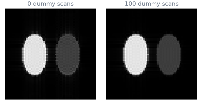
closed form: short T1 over long T1, 3.73
  0 dummy scans: short T1 over long T1, 3.56
100 dummy scans: short T1 over long T1, 3.73

With dummy scans, the images show the T1 weighting of a spoiled gradient echo at a short TR, at the ratio the closed form gives. Without them, each line is acquired on the way to steady state: the long-T1 ellipse is brighter than in steady state, and its signal changes from line to line, which leaves ghosts along the phase-encoding axis. A scan on the Fourier engine tests the sequence’s contrast as well as its trajectory and its reconstruction.

Conversion check

validate() compares the gradients the sequence asks for with a second rendering. Without a recording of a scanner playing it, the rendering is the cache’s own waveforms. Agreement establishes that the conversion kept the sequence; it does not establish that a scanner plays it.

from pulserver.validate import validate

print(validate(paths[0], system=system))

the sequence agrees with the ir waveforms
  gx     largest difference 9.542e-06 of 38.79 (0.00%)
  gy     largest difference 7.34e-08 of 21.35 (0.00%)
  gz     largest difference 3.35e-10 of 35.63 (0.00%)