Extended phase graphs#
Three pulses generate five echoes, and a train of a hundred generates far more than a hundred. A refocused train, a gradient-echo steady state, a fingerprinting schedule: in each, what you sample is not one decaying magnetization but a sum over routes through the pulses and the gradients, each of which has spent a different amount of time transverse and a different amount parked along the field. The extended phase graph (EPG) is the accounting that keeps those routes straight, and it is what TorchSim evaluates. Weigel [2] is the introduction to read alongside this one.
The magnetization is decomposed into configuration states, and three operators act on them:
Transition – an RF pulse, which mixes the transverse and longitudinal families within an order and never moves a state between orders.
Shift – a gradient, which moves transverse states between orders and mixes nothing.
Evolution – relaxation and precession between events. Decay reaches every state; recovery toward equilibrium reaches order zero alone.
A sequence is those three alternating, and the signal is read off the states wherever it samples. This page is the physics; how it is realized – the events, the kernels, the derivatives – is How TorchSim runs it.
Dephasing#
A voxel is not one magnetization vector. It is an ensemble of isochromats, and a gradient gives each of them a Larmor frequency that depends on where it sits. Over an interval the phase they acquire is linear in position, so the ensemble winds into a helix, and the signal – which is the sum over the voxel – falls away as the helix tightens. Nothing has been lost: the magnetization is still there, wound up, and a gradient of the opposite sign will bring it back.
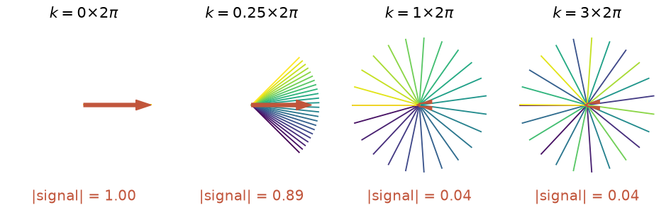
Isochromats across one voxel, in the transverse plane, after gradient areas winding zero, a quarter, one and three turns across it. The red arrow is their sum, which is all a receiver ever sees. Past one full turn the sum is effectively zero and stays there, while the ensemble underneath it is perfectly ordered.#
The winding is measured by \(k = \gamma \int G\,\mathrm{d}t\), the same quantity as the k-space coordinate of imaging. It is the natural coordinate for this problem: a gradient does one thing to the ensemble, which is to move \(k\).
Configuration states#
Because the phase is linear in position, the transverse magnetization across the voxel is a sum of spatial harmonics, and each harmonic is labelled by its winding \(k\). Writing \(M^{+}(r) = M_x + iM_y\) and taking its Fourier transform over the voxel gives the configuration states
and the states are the whole description: the spatial profile is recoverable from them, and the measured signal is exactly the coherent one, \(\tilde F^{+}(0)\). This is the configuration-state treatment of echo trains introduced by Hennig [1], in the notation of Weigel’s review [2], which the rest of this page follows.
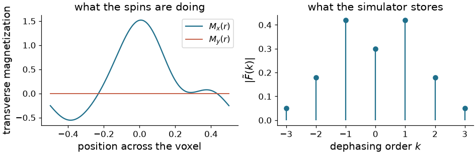
Left, the transverse magnetization across a voxel part-way through a sequence – the thing an isochromat summation would need thousands of samples to represent. Right, the same state as configuration amplitudes. A sequence that winds by whole turns populates only integer orders, so a handful of numbers carries the voxel exactly rather than approximately.#
This is the move that makes EPG cheap. An isochromat simulation pays for spatial resolution it does not care about; the phase graph pays for the number of orders the sequence actually populates, which is small and which you can count in advance from the gradients.
Three families of state#
Transverse magnetization is complex, and its two conjugate halves behave differently under a gradient, so they are tracked separately as \(\tilde F^{+}(k)\) and \(\tilde F^{-}(k)\). Longitudinal magnetization is modulated across the voxel too – a pulse can store a wound-up transverse state along \(z\), where it neither dephases further nor decays with \(T_2\) – so it has configurations of its own, \(\tilde Z(k)\). Those three families at each integer order are the entire state of a voxel.
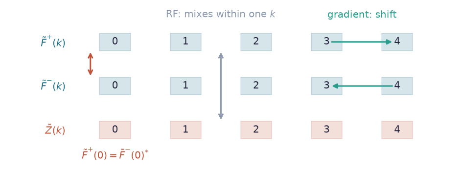
The state of a voxel: three families over the integer dephasing orders. A gradient moves populations along the rows in opposite directions; an RF pulse mixes them within a column and never moves an order. At order zero the two transverse families are the same information, since \(\tilde F^{+}(0)\) and \(\tilde F^{-}(0)\) are complex conjugates of one another – which is why order zero needs a rule of its own in every implementation.#
The transition and shift operators act on that grid.
RF pulses#
A hard pulse of flip angle \(\alpha\) and phase \(\varphi\) acts identically on every order – it cannot move magnetization in space, only turn it – so it is one 3x3 matrix applied to each column:
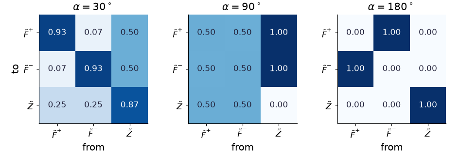
The magnitude of \(\mathbf{T}\) at three flip angles. A 180 degree pulse swaps the two transverse families outright – perfect refocusing – and inverts \(\tilde Z\). A 90 degree pulse splits every state three ways: it refocuses half, leaves half dephasing, converts all longitudinal magnetization into transverse, and stores half of the transverse along \(z\). A small pulse mostly leaves things where they were, which is why a low-flip train carries so many pathways at once.#
The off-diagonal entries are the entire reason echoes proliferate. Every pulse that is neither 0 nor 180 degrees splits each populated state into three, so the number of live pathways grows with each pulse until relaxation and truncation kill the weakest.
Gradients#
A gradient’s only effect is to change the winding, which in this basis is a shift by whole orders:
with the longitudinal states untouched, because they carry no phase to wind.
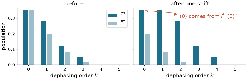
One unbalanced gradient, before and after. Everything transverse moves up one order in \(\tilde F^{+}\) and down one in \(\tilde F^{-}\). The order-zero entry is the interesting one: it is refilled from the conjugate of what was at order zero in the other family, which is the bookkeeping that makes rephasing come out right and is the single place a shift is not just a memory move.#
In TorchSim the shift is what an operator such as Dephase plays, and one
shift is one crusher or one unbalanced readout gradient. Ideal spoiling –
Spoil – is the other option: discard every transverse order instead of
winding it on, which is what a spoiled gradient echo assumes its spoiler and
its RF phase cycling achieve together.
Relaxation and recovery#
Between events, transverse states decay by \(E_2 = e^{-\Delta t / T_2}\) and longitudinal states by \(E_1 = e^{-\Delta t / T_1}\). Recovery toward equilibrium, though, is spatially uniform: it adds magnetization with no modulation at all, so it enters \(\tilde Z(0)\) alone.
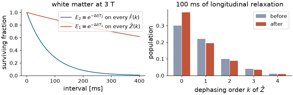
Left, the two attenuation factors for white matter at 3 T. Right, what 100 ms of longitudinal relaxation does to a set of \(\tilde Z\) states: every order is scaled by \(E_1\), and only order zero gains the \(M_0(1 - E_1)\) that regrowth supplies. A modulated longitudinal state decays toward zero, not toward equilibrium, because equilibrium has no modulation to relax into.#
Reading the graph#
Plotting \(k\) against time turns a sequence into a picture. Between pulses every transverse pathway moves at a constant rate set by the gradients; at each pulse it may continue, reverse, or be parked along \(z\) until a later pulse brings it back. Wherever a transverse pathway crosses \(k = 0\) there is an echo, and the sample is the sum of every pathway crossing at that moment.
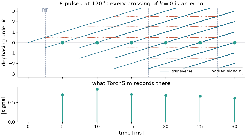
Above, the phase graph of six refocusing pulses: solid lines are transverse pathways, dotted lines are magnetization parked along \(z\) between pulses, dashed verticals are the pulses. Below, what TorchSim records at those crossings. From the fourth pulse on, the sampled signal contains direct spin echoes and stimulated echoes at once – pathways that spent one or more intervals longitudinal, and so were spared \(T_2\) decay while they were there.#
The diagram is what makes EPG a way of thinking and not only of computing. Refocusing angle, echo spacing, spoiler size and RF phase all change the graph in ways you can see before you simulate anything.
Stimulated echoes#
With anything other than exact 180 degree refocusing, an echo train is not a mono-exponential. Stimulated-echo pathways spend part of their life along \(z\), so they arrive with less \(T_2\) decay than their echo time suggests, and the train picks up oscillations at its start and a long tail at its end.
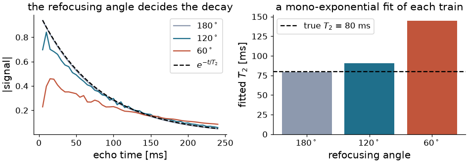
Left, a 48-echo train at three refocusing angles beside \(e^{-t/T_2}\). Right, the \(T_2\) a mono-exponential fit of each train returns. Only the 180 degree train recovers the true value; the low-flip trains – which is what a real sequence plays, to stay inside SAR – are biased by tens of percent. This is the practical case for simulating the pathways rather than assuming the decay.#
Configuration orders to carry#
A sequence populates a bounded set of orders: each shift moves the ladder by
one, so after \(n\) shifts nothing beyond order \(n\) exists, and
attenuation makes the far orders negligible long before that. You choose how
many to carry with states= (or nstates= per call), and TorchSim sizes it
from the winding the sequence declares when you do not.
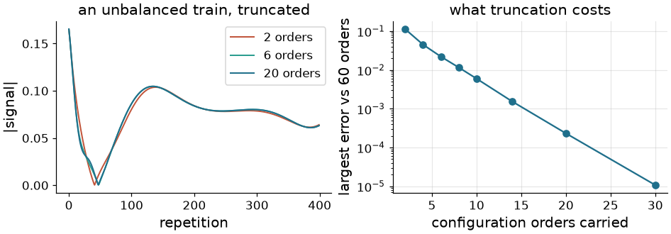
Left, an unbalanced fingerprinting train carried with 2, 6 and 20 orders. Right, the largest error against a 60-order reference. The error falls geometrically: a handful of orders is qualitatively wrong, a dozen or two is right to well below the noise of any real measurement. Truncating is not an approximation you have to accept blindly – it is a convergence you can measure for your own sequence with two calls.#
Diffusion and flow#
A state at order \(k\) is wound up in space, and anything that moves spins around inside the voxel scrambles that winding. Over an interval a state accumulates a diffusion b-factor weighted by \(k^2\) while it is longitudinal, and by \(k^2 + k + 1/3\) while it is transverse and winding through the interval [2]. Order zero is untouched, which is why diffusion enters through the pathways rather than as a single exponential on the signal.
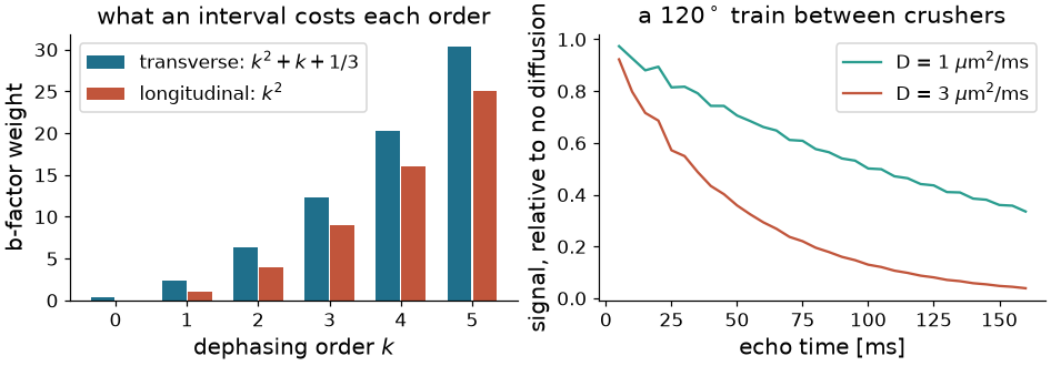
Left, what one interval costs each order. Right, a 120 degree train played between crushers winding 20 turns across a millimetre voxel, at two diffusion coefficients, relative to the same train with no diffusion. The attenuation is neither exponential in time nor uniform across echoes, because the pathways contributing to each echo have spent different amounts of time at different orders. Coherent flow enters the same way but as a phase per order rather than an attenuation, and washout replaces the excited spins outright.#
Both effects need geometry the sequence has to declare – how far a crusher winds and across what voxel – because a dephasing order is only a b-factor once you know the gradient behind it.
Second pool#
Tissue is not one proton pool. TorchSim carries the two extensions of the EPG formalism that matter in practice, both from Malik et al [3]: a semisolid pool that RF saturates through its absorption lineshape and that exchanges longitudinal magnetization with the free water (magnetization transfer), and a chemically exchanging pool that has transverse states of its own and sits at a frequency offset (Bloch-McConnell). Exchange couples states of the same family and the same order, so the phase-graph structure is unchanged: what changes is that relaxation and exchange are one combined operator, since the two do not commute.
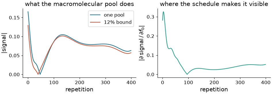
Left, a fingerprinting trajectory on white matter, with and without a bound pool holding 12% of the magnetization. The pool is never sampled – it has no transverse magnetization to detect – and it still moves the trajectory by a sizeable fraction of its peak, so a dictionary built from the single-pool model is wrong in a way no amount of matching recovers. Right, the derivative of the signal with respect to the bound fraction, which is what says whether the schedule can estimate it rather than merely be affected by it.#
Assumptions#
EPG is exact for what it models. It assumes the dephasing within a voxel is linear in position, so that a gradient is a shift; sequences whose gradients are unbalanced by non-integer amounts, or whose voxels contain their own strong field variation, need the orders to be interpreted with care. It treats an isochromat’s off-resonance as a constant precession rather than as a distribution, so a spread of field across the voxel is not something the states carry.
TorchSim applies that spread to the samples instead. t2_prime_ms sets a
Lorentzian population of frequencies, half-width \(1 / T_2'\) in angular
frequency, whose average over the voxel is \(e^{-|\tau| / T_2'}\) in the time
\(\tau\) a sample has gone
unrefocused – so a gradient echo decays at \(T_2^*\), a spin echo is left at
\(T_2\), and the decay grows and recovers either side of each echo. It asks the
sequence to wind at one steady rate, which is the condition under which a
configuration order stands for elapsed time as well as for area; a balanced
train does not, and needs a spread of b0_hz across voxels as before.
Pulses are instantaneous rotations unless you say otherwise. A real slice-selective pulse acts under its gradient, so what it does depends on position within the slice; TorchSim can carry that exactly by integrating the pulse ahead of time, which is the hybrid Bloch-EPG picture of Guenthner et al [4] and is described in How TorchSim runs it.