Note
Go to the end to download the full example code or to run this example in your browser via Binder.
Basic Usage#
The scope of this notebook is to showcase the basic functionalities of Torchsim, including how to simulate a signal, calculating derivatives etc.
This example uses a fast spin echo that ships with TorchSim.

import math
import time

import numpy as np
import torch

import torchsim
from torchsim.simulators import FSESimulator
Forward simulation#
First, we need to create a Simulator object instance. The constructor accepts the sequence parameters (in this example, number of echoes and echo spacing) and the tissue properties (T1, and T2).
The simulator is parallelized: if N (T1, T2) pairs are provided, the corresponding N signals are computed in parallel. Properties support broadcasting: if we pass a list of T2s but just a single T1, the same T1 is used for all atoms.
Changing the system parameters (e.g., simulating a refocusing train with 60° flip angle) will affect the resulting signal evolution
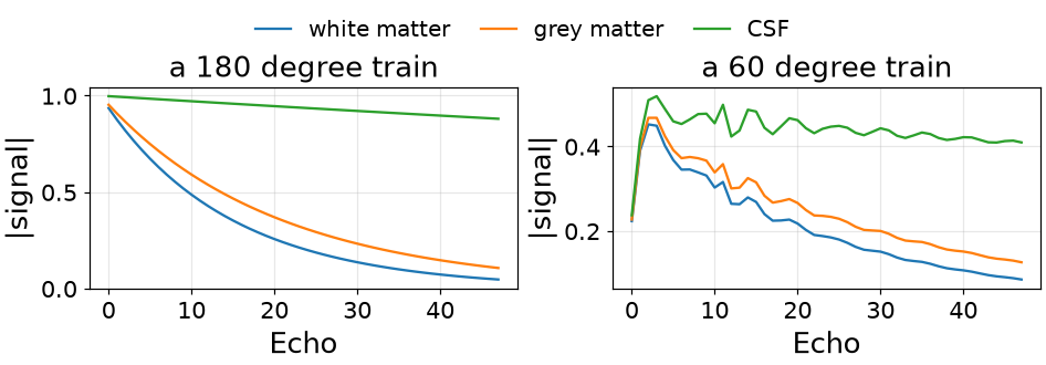
<matplotlib.legend.Legend object at 0x7f1b8e5f86e0>
Derivative with respect to tissue parameters#
Torchsim allows to efficiently evaluate the derivative
of the signal wrt input parameters, via jacobian().
The desired derivatives can be specified by string:
signal, dT2 = simulator.jacobian("T2", flip=flip) # dT2 is (3, 48) too
Since the number of echoes is typically much larger than the number of differentiation parameters, forward mode differentiation is more efficient than the more common backward propagation.
Here you can see a comparison with finite differences derivatives:
largest disagreement with a 1.0 ms step: 7.70e-03
Approaching steady state#
Everything so far started from equilibrium. A scanner does not: it plays the train over and over, and what it records is the state the train has settled into. Reaching that by playing it out is hundreds of repetitions, every one of them the full cost of the sequence.
repetitions="auto" reads the limit off a handful of playings instead. A
settled signal is a constant plus decaying modes, so finitely many terms fix
where it is going, and the answer is the one that running there arrives at.
one playing          0.78021
repetitions="auto"   0.05895
200 playings         0.05895
the last two agree to 4.7e-02
The first playing is wrong by a fraction that a short TR makes large, which is what a simulation of a steady-state sequence gets wrong if it starts from equilibrium and stops. Every shipped simulator takes the setting, and it costs a fraction of what running there costs.
Functional wrapper#
Every sequence that ships also has a function, for the case where there is
nothing to reuse: it takes the protocol and the tissue together, returns the
signal, and returns the derivative too if diff names a property. It is
the object above with the construction folded in, so the answer is the same
to the bit.
signal, dT2 = torchsim.fse_sim(
    flip=flip, ESP=ESP_MS, TR=3000.0, T1=T1_MS, T2=T2_MS, diff="T2"
)
agrees with the simulator to 0.0e+00
Reach for it when a sequence is simulated once and nothing about it is being varied. The object is what a loop wants: it resolves the event stream on its first call and rebinds only the numbers that change afterwards, which is worth about eight times the whole call to a design or a dictionary sweep.
Performance tweaking#
Everything so far took the defaults. Four settings decide what the run costs and how exact it is, and each is given to the constructor or to the call.
states is how many configuration orders are carried. A refocused train
winds one order per interval, and a pulse that is not a perfect 180 degrees
splits the magnetization down every pathway those orders describe, so the
answer is only as good as the number kept. Too few is a wrong answer rather
than a slow one. Held against a train carrying far more than it needs:
 4 orders   0.0e+00 from converged
10 orders   0.0e+00 from converged
16 orders   0.0e+00 from converged
32 orders   0.0e+00 from converged
48 orders   0.0e+00 from converged
It lands exactly at forty-eight, which is the number of echoes: a train that winds one order per interval can populate one more pathway per echo and no more, so carrying more orders than the train has intervals changes nothing. A spoiled sequence is the other case – it discards the transverse orders every repetition, so a handful is enough however long it runs.
The shipped default is chosen for the refocused trains these simulators are written for, and a 60 degree train is not one of them. It is the first setting to raise when a signal looks wrong late in an echo train, and the check above – run once against a larger number – is how you find out rather than assume.
A simulator is worth holding on to. The structure of a sequence – the order of its events, which of them record, how far it winds – is settled the first time it runs and the numbers are rebound onto it afterwards, so a sweep that changes only flip angles never walks the event stream again. That happens by itself; what it is worth grows with the sequence, and a 500-repetition fingerprinting schedule is where it decides whether a dictionary sweep takes minutes or hours.
held = FSESimulator(ESP=ESP_MS, TR=3000.0, T1=T1_MS, T2=T2_MS)
rebuilt = FSESimulator(ESP=ESP_MS, TR=3000.0, T1=T1_MS, T2=T2_MS)

for name, candidate in (("held", held), ("rebuilt anew", rebuilt)):
    candidate.simulate(flip=flip)  # the first call is where the structure is read
    start = time.perf_counter()
    for _ in range(20):
        if name != "held":
            candidate = FSESimulator(ESP=ESP_MS, TR=3000.0, T1=T1_MS, T2=T2_MS)
        candidate.simulate(flip=flip)
    print(f"  {name:14s} {1e3 * (time.perf_counter() - start) / 20:6.2f} ms a call")
held             0.80 ms a call
rebuilt anew    11.61 ms a call
execution says where the work goes. "auto" weighs the problem against
what the cards have free – work too small to repay a launch stays on the
host, work that fits crosses in one piece, work that does not is streamed
through in chunks. Naming a device insists on it, and a block settles it for
everything inside:
with torchsim.execution("cpu"):
    on_the_host = simulator.simulate(flip=flip)

print(
    f"  forced onto the host, agrees to {float((on_the_host - signal_ref).abs().max()):.1e}"
)
forced onto the host, agrees to 0.0e+00
stream and budget_bytes are for a volume rather than a dictionary:
the first insists the run be cut into chunks even where it would have fit,
the second caps what a chunk may hold. A whole-brain map at a hundred
thousand voxels is the case they exist for, and it is written like this:
if torch.cuda.is_available():
    with torchsim.execution("cuda", stream=True, budget_bytes=1 << 28):
        streamed = simulator.simulate(flip=flip)
    agreement = float((streamed.cpu() - signal_ref).abs().max())
    print(f"  streamed through a card in 256 MiB chunks, agrees to {agreement:.1e}")
else:
    print("  no card here, so the streamed run is skipped")
no card here, so the streamed run is skipped
Simulating a sequence you did not write#
Every call so far named the sequence: ESP, TR, the flip train. That
is fine when you wrote it, and wrong when it came from somewhere else – a
scan does not need its parameters retyped, it needs them read.
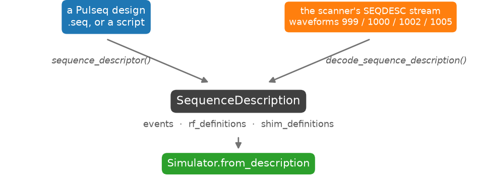
The MRD client streams a sequence description, having taken it from the Pulseq sequence the scanner is running. It is a repetition’s worth of events: time passing, an RF pulse, an ADC window, each with a timestamp and the numbers that kind of event carries, plus the pulse shapes and transmit shims they name.
Echo spacing, echo train length, refocusing angle, TR and pulse shapes are all in there. Nothing about the sequence has to be given again.
described = simulator.describe(flip=flip, ESP=ESP_MS, TR=3000.0)
145 events over 3000 ms, 1 pulse shape, 0 shims
You do not have to read it. describe here only shows what a stream looks
like; plot() draws one, which is the way
to check that a layout laid down what you meant.
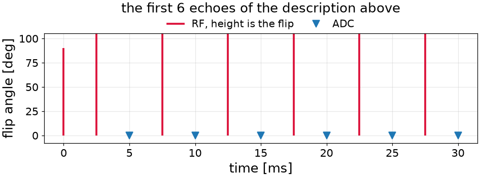
[<matplotlib.legend.Legend object at 0x7f1b8e4dcf50>]
A description normally arrives; it is not typed. Writing one by hand once is
worth it only to see that there is nothing else in it –
from_operators() lays them out.
by_hand = torchsim.SequenceDescription.from_operators(
    torchsim.Excitation(math.pi / 2, math.pi / 2),
    *[
        part
        for _ in range(ECHOES)
        for part in (
            torchsim.Delay(0.5 * ESP_MS * 1e-3),
            torchsim.Refocusing(math.radians(60.0), 0.0),
            torchsim.Delay(0.5 * ESP_MS * 1e-3),
            torchsim.Readout(0.0),
        )
    ],
)

print(
    f"  written by hand: {len(by_hand.events)} events over "
    f"{by_hand.tr_duration_us * 1e-3:.0f} ms"
)
written by hand: 193 events over 240 ms
from_description() runs one, and the only
thing given to it is the tissue. The events are already concrete – each
carries the action word saying whether it winds, spoils or records – so no
layout is walked and no sequence parameter is inferred.
Which simulator you call it on is the whole of what you choose, and it is not a formality. A description says an RF pulse was played, tagged with the use its designer gave it, and an ADC window was opened. It says nothing about the gradients between them, because the transport carries none.
The dephasing lives in the handlers instead: a refocused train crushes
either side of its refocusing pulses, an unbalanced one winds an order after
every sample, a spoiled one discards the transverse states. Naming
FSESimulator is how you say which of those the events are to be read as.
from_stream = FSESimulator.from_description(described, states=10, T1=T1_MS, T2=T2_MS)
streamed_signal = from_stream.simulate()
It differentiates like anything else, because the derivative follows from the events and not from who wrote them:
_, streamed_dT2 = from_stream.jacobian("T2")
signal (3, 48), dT2 (3, 48)
One thing to know when comparing it against the shipped simulator: a
description carries the events, and a simulator may carry physics around
them. FSESimulator folds in the recovery
between one train and the next in closed form, which is not an event and so
is not in the stream. The shape of the train is the same; the driven
equilibrium the shipped object adds does not come along.
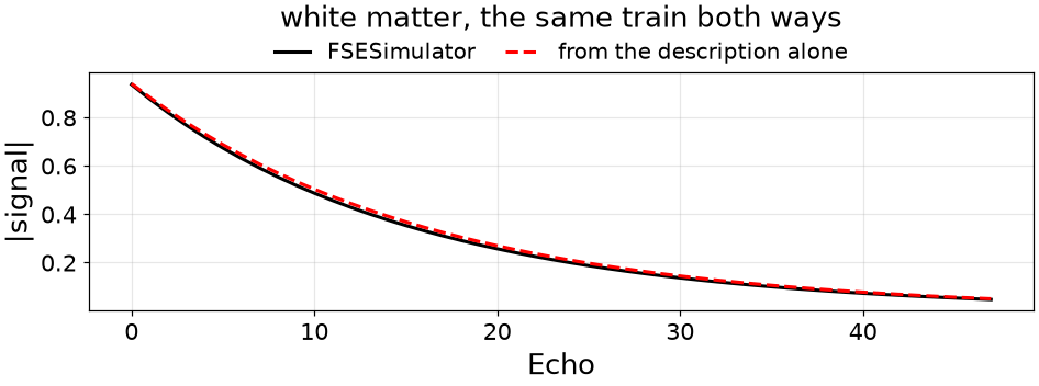
[<matplotlib.legend.Legend object at 0x7f1b8df55250>]
From a Pulseq file#
The stream a scanner sends is read off the Pulseq sequence it is running, so
the same events can be read from the .seq file directly – which is what
to do when the scan has not been run yet. The file is parsed by pypulseq,
which also computes its trajectory: pip install torchsim[pulseq].
The file states how many blocks one repetition holds, in its TRSize
definition, so nothing is searched for. What is read off the trajectory is
what Pulseq does not write down: which ADC sample each readout passes
through k = 0 in, which is the echo the timestamp goes on.
train = FSESimulator.from_pulseq(SEQ_FILE, states=20)
from_file = train.simulate(T1=T1_MS, T2=T2_MS)
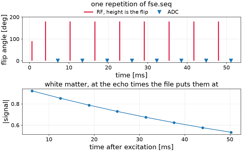
read from fse.seq:
  25 events over 2053 ms
  8 echoes, 6.28 ms apart
  2 pulse shapes
Echo spacing, echo train length, refocusing angle and pulse shapes were never named. The two things given were the tissue and which simulator to read the events as.
Next steps#
The derivative with respect to tissue is what a fit descends and what a model-based reconstruction pushes through an encoding operator; the parameter inference and model-based imaging notebooks do both. Differentiating with respect to the schedule instead is what designs a protocol, and is the subject of the sequence optimization notebooks.
When the sequence you want is not one of the ones that ship, the next notebooks say what to write instead.
Total running time of the script: (0 minutes 6.582 seconds)
