Writing a Signal Model

The scope of this notebook is to write a simulator TorchSim does not ship.

There are two things to say. Which operator plays each kind of event – what an excitation is, what a sample is – and what order they are played in. The base class does the rest: it resolves the layout into an event stream, rebinds values onto it, holds the derivatives, places the work on a device, and reads a sequence back from a description a scanner streamed.

The base class, and the operators a layout is written from.

import numpy as np
import torch

from torchsim import (
    Delay,
    Excitation,
    Inversion,
    SPGRReadout,
    SSFPFidReadout,
    Spoil,
)
from torchsim.model import Simulator

Handlers

A simulator says what plays each kind of event by naming it. The five readouts are what distinguishes one steady-state family from another: an SSFPFidReadout() winds one configuration order after every sample, an SSFPEchoReadout() winds it before, an SPGRReadout() spoils, a bSSFPReadout() leaves the states where they were, and an FSEReadout() samples a spin echo the refocusing pulses have already crushed around.

Naming one is the whole of choosing between them, and it is also what says how an arriving stream is to be read – the transport carries no gradients, so the handler is where the dephasing lives.

Nothing is said here about the tissue. Every property a voxel has can be given to any simulator, and giving one is what turns its term on.

Layout

An Simulator is the protocol. You do not write timestamps: layout returns the operators of one repetition in order, and the simulator turns the span each one holds into the timestamps a description carries.

self.operators is the handler set named above. What layout produces is an event stream whose events carry their own action word, and from there the path is the fused one – packing, the feature mask, offload and sharding.

class SSFPMRF(Simulator):
    """An Inversion, then one Excitation and one sample per repetition."""

    excitation = Excitation
    inversion = Inversion
    readout = SSFPFidReadout
    states = 10

    def layout(self, *, flip, TR, TI=0.0):
        """Return one repetition's operators, in the order they are played."""
        angles = torch.deg2rad(torch.as_tensor(flip))
        parts = [self.operators.inversion(duration_s=TI * 1e-3)]
        for index in range(angles.numel()):
            parts.append(self.operators.excitation(angles[index]))
            parts.append(self.operators.readout(duration_s=TR * 1e-3))
        return parts

Running the simulator

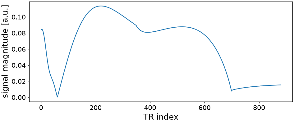
Property and sequence arguments are given together and told apart by properties. A scalar property is one voxel; an array is a map, and every voxel runs at once.

flip = np.concatenate(
    (np.linspace(5.0, 60.0, 350), np.linspace(60.0, 1.0, 350), np.ones(180))
)

sequence = SSFPMRF(flip=flip, TR=10.0, TI=20.0)
signal = sequence.simulate(T1=1000.0, T2=100.0)

Text(30.823120572916668, 0.5, 'signal magnitude [a.u.]')

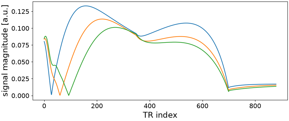
The same call over a parameter map returns one row per voxel:

signals = sequence.simulate(
    T1=torch.tensor([500.0, 1000.0, 1500.0]),
    T2=torch.tensor([50.0, 100.0, 150.0]),
)

Text(30.823120572916668, 0.5, 'signal magnitude [a.u.]')

Forward-mode derivatives

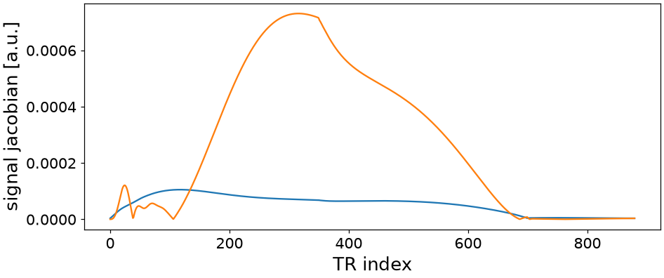
A Bloch simulation records far more samples than it takes parameters, so a derivative with respect to tissue is cheapest taken forwards: one directional derivative per property yields every voxel’s derivative at once, and the cost is one pass per property rather than per voxel.

That is what jacobian() does. A single name collapses the parameter axis; a sequence of names keeps it.

signal, jacobian = sequence.jacobian(("T1", "T2"), T1=1000.0, T2=100.0)

Text(30.823120572916668, 0.5, 'signal jacobian [a.u.]')

Reverse-mode derivatives

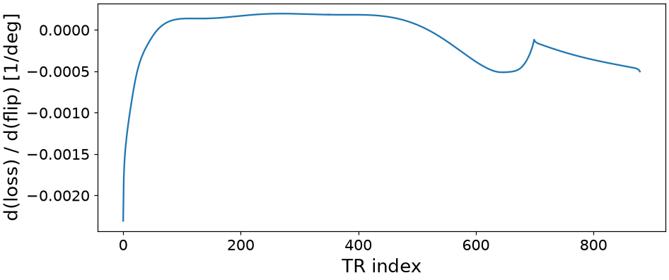
The simulator optimization problem runs the other way: one scalar cost, many sequence parameters. That is reverse mode, and it is deliberately not wrapped – build a cost on the signal and call backward(). The engine reads which of its inputs carry a gradient and picks its kernel from that, so a layer here would only hide the choice.

schedule = torch.tensor(flip, dtype=torch.float32, requires_grad=True)
recorded = sequence.simulate(T1=1000.0, T2=100.0, flip=schedule)
loss = -recorded.abs().square().sum()
loss.backward()

Text(30.823120572916668, 0.5, 'd(loss) / d(flip) [1/deg]')

Additional physics

Nothing was declared about the tissue, and nothing had to be. Naming a property in the call is what turns its term on, so a second exchanging pool is four more names in the call and no change to the simulator:

two_pool = sequence.simulate(
    T1=1000.0,
    T2=100.0,
    poolB_fraction=0.2,
    poolB_exchange=20.0,
    poolB_T1=500.0,
    poolB_T2=20.0,
)

a second pool moves the train by 17.9%

What the whole vocabulary is, and what each term does to a train, is the expanded-physics example.

Validation against a closed form

A fingerprinting train has no closed form to check against, so here is a second simulator that does. Saturation recovery destroys whatever magnetization was there, waits, and reads what has come back – and what it reads at a saturation time is \(M_0 \sin\alpha \, (1 - e^{-T_S/T_1})\), because the saturation leaves nothing behind and the recovery is undisturbed until the readout.

The state machine has never been told what sequence these events add up to. It plays them, so agreeing with the closed form is a check rather than a tautology.

@ composes two operators into one, so the saturation reads as the single thing a physicist would name rather than as a pulse and a spoiler.

class SaturationRecovery(Simulator):
    """Saturate, wait, read what recovered -- once per saturation time.

    Parameters
    ----------
    TS : array-like
        Saturation times, in milliseconds, one per block.
    flip : float
        The readout flip angle, in degrees.
    phases : float or array-like, optional
        The readout phase, in degrees.
    """

    excitation = Excitation
    readout = SPGRReadout
    # Every block begins by destroying the transverse magnetization, so nothing
    # is carried in a dephased configuration and one order is the whole state.
    states = 1

    def layout(self, *, TS, flip, phases=0.0):
        """Return one saturate-wait-read block per saturation time."""
        waits = torch.atleast_1d(torch.as_tensor(TS)) * 1e-3
        angle = torch.deg2rad(torch.as_tensor(flip)).broadcast_to(waits.shape)
        turn = torch.deg2rad(torch.as_tensor(phases)).broadcast_to(waits.shape)

        saturate = Excitation(torch.pi / 2) @ Spoil()
        parts = []
        for index in range(waits.numel()):
            parts.append(saturate)
            parts.append(Delay(waits[index]))
            parts.append(self.operators.excitation(angle[index], turn[index]))
            parts.append(self.operators.readout(turn[index]))
        return parts

SATURATION_TIMES = torch.tensor([50.0, 100.0, 200.0, 400.0, 800.0, 1600.0, 3200.0])
FLIP_DEG = 10.0
T1_MS = torch.tensor([830.0, 1330.0, 4000.0])
NAMES = ("white matter", "grey matter", "CSF")

recovery = SaturationRecovery(TS=SATURATION_TIMES, flip=FLIP_DEG)
recovered = recovery.simulate(T1=830.0, T2=80.0, M0=1.0).abs()
closed_form = torch.sin(torch.deg2rad(torch.tensor(FLIP_DEG))) * (
    1.0 - torch.exp(-SATURATION_TIMES / 830.0)
)

times = torch.logspace(1.3, 3.7, 60)
curves = SaturationRecovery(TS=times, flip=FLIP_DEG).simulate(
    T1=T1_MS, T2=torch.tensor([80.0, 110.0, 2000.0]), M0=1.0
)

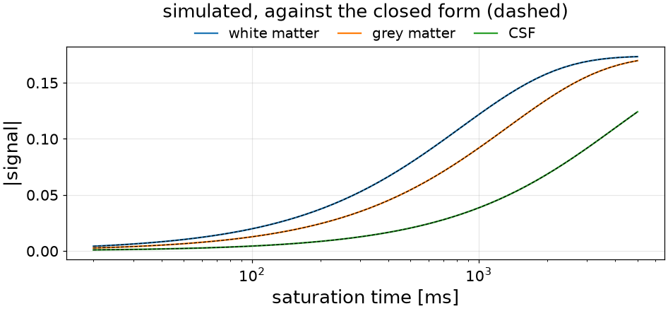
  largest disagreement with the closed form: 7.45e-09

[<matplotlib.legend.Legend object at 0x7f1b947d0110>]

Inspecting the event stream

describe() returns the event stream, which is the same object a sequence arriving from a scanner is read into: a timestamp and an action word on every event. It is worth looking at once, because a sequence that plays the wrong thing is far easier to see here than in the signal it produces.

description = recovery.describe(TS=SATURATION_TIMES, flip=FLIP_DEG)

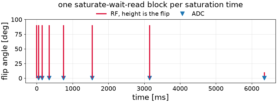
  49 events, 6350 ms long

[<matplotlib.legend.Legend object at 0x7f1b8ddd2810>]

Building from a description

A description that came from somewhere else – an MRD file, a Pulseq export, a scanner’s own stream – becomes a simulator through from_description(). No layout is walked: the events are re-emitted through this model’s handlers, which is what puts the gradients back that the transport does not carry.

It does not reproduce this sequence exactly, and the gap is the lesson. A handler reinstates what a pulse or a sample implies; the spoiler inside the saturation block is neither, so nothing reinstates it – and a stream arriving from a scanner could not have carried it either. A preparation that has to survive the round trip belongs in a pulse the wire can name.

arrived = SaturationRecovery.from_description(description, states=1)

the same stream, read back through the handlers, differs by 5.3e-01

Functional wrapper

The shipped models come with one, and yours can too:

def ssfp_mrf_sim(flip, TR, T1, T2, TI=0.0, diff=None):
    """Simulate an inversion-prepared SSFP train, and differentiate it."""
    sequence = SSFPMRF(flip=flip, TR=TR, TI=TI)
    if diff is None:
        return sequence.simulate(T1=T1, T2=T2)
    return sequence.jacobian(diff, T1=T1, T2=T2)


signal, jacobian = ssfp_mrf_sim(flip, 10.0, 1000.0, 100.0, diff=("T1", "T2"))
# signal is (repetitions,); jacobian is (2, repetitions), one row per property