MP2RAGE lookup table

The scope of this notebook is to map T1 from a two-block MP2RAGE, by interpolating along a curve and by matching the same curve, and to sweep the number of points to show which of the two is limited by it.

With a single unknown a dictionary degenerates: the atoms lie on a curve rather than filling a space. Interpolating between the two nearest then costs nothing and takes the grid spacing out of the answer, which is what LookupTable does.

The problem is stated over a simulator carrying the sequence and filled in by an estimator. execution() decides where that work runs, and the timings below are taken inside it.

import time

import numpy as np
import torch

import torchsim
from torchsim.estimators import DictionaryMatcher, LookupTable
from torchsim.simulators import MP2RAGESimulator

Phantom

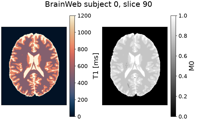
BrainWeb subject 0, slice 90: an axial slice at 1 mm through the lateral ventricles. BrainWeb publishes fuzzy memberships rather than labels, so each voxel holds a fraction of each tissue, and the relaxation times are weighted by those fractions. A third of the voxels are mixtures, so the truth is a continuum and not four values.

Text(0.5, 0.9901188654526398, 'BrainWeb subject 0, slice 90')

Protocol

One inversion, two spoiled gradient-echo blocks read at two inversion times. Each block samples the centre of k-space of its own shot train, so a voxel contributes two numbers. The train spoils after every readout, so T1 is the only tissue property that moves them.

PROTOCOL = dict(
    TI=(800.0, 2700.0),
    flip=(4.0, 5.0),
    TRspgr=6.7,
    TRmp2rage=6000.0,
    nshots=128,
)
INVERSION_EFFICIENCY = 0.96

simulator = MP2RAGESimulator(**PROTOCOL, inv_efficiency=INVERSION_EFFICIENCY)

Signal curve

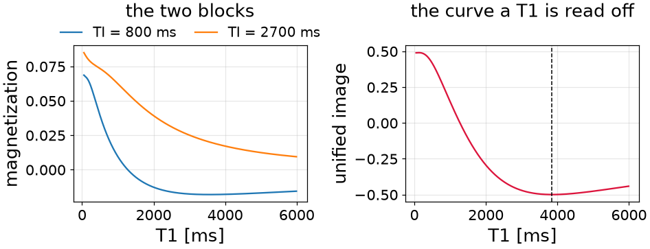
Neither block alone says T1: both carry the proton density and the receive gain. The unified combination divides that scale out, leaving a number between -0.5 and 0.5 that depends on T1 alone. Which combination is monotonic belongs to the sequence, so it is given rather than assumed.

def unified(blocks):
    """The MP2RAGE unified image: scale-free, and a function of T1 alone."""
    return (blocks[..., 0] * blocks[..., 1]) / blocks.square().sum(-1).clamp_min(1e-12)

The curve is not monotonic over every T1, and where it turns back it has no inverse. The table keeps the longest monotonic run and reports what it spans, so the invertible range is a number rather than an assumption.

sweep = torch.arange(50.0, 6000.0, 10.0)
curve = unified(simulator.simulate(T1=sweep, M0=1.0))

[<matplotlib.legend.Legend object at 0x7f1b8cb7b4d0>]

Measurement

Both blocks, at the true T1 and proton density of every brain voxel, with noise at half a percent of the peak magnetization.

clean = simulator.simulate(T1=truth, M0=density)
NOISE_STD = float(0.005 * clean.abs().max())

generator = torch.Generator().manual_seed(42)
measured = clean + NOISE_STD * torch.randn(clean.shape, generator=generator)

Two estimators

Both are given the same T1 grid. The match scores the two-block signal against every atom and takes the nearest; the table reduces both blocks to the unified number and interpolates along the curve, so combine is all it is told. Neither is given the range in advance.

grid = torch.linspace(50.0, 6000.0, 60)

table = LookupTable(simulator.bind(M0=1.0), combine=unified).fit(T1=grid, seed=0)

maps = table.map(measured)  # {"T1": ...}, one value per voxel

match = DictionaryMatcher(simulator.bind(M0=1.0)).fit(T1=grid, seed=0)

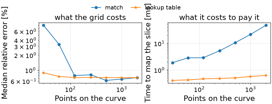
Sweeping the grid separates the method from the sampling. Times are the best of three passes over the slice.

 points     match     table     match     table
            error     error      time      time
-----------------------------------------------
     30     7.93%     0.88%     1.9ms     0.4ms
     60     3.29%     0.75%     2.8ms     0.4ms
    120     0.78%     0.71%     2.9ms     0.5ms
    250     0.80%     0.71%     5.2ms     0.5ms
    500     0.62%     0.71%    10.6ms     0.5ms
   1000     0.66%     0.71%    21.8ms     0.6ms
   2000     0.71%     0.71%    47.7ms     0.6ms

The table is at its floor from the coarsest grid and does not move again. The match starts an order of magnitude worse and climbs to the same place, paying for it in points: its search is one comparison per atom per voxel, where the table’s binary search grows with the logarithm.

The floor both reach is the noise. A fine enough grid matches a table exactly; the table’s advantage is that it was never told how fine.

<matplotlib.legend.Legend object at 0x7f1b8cb7ab10>

Maps

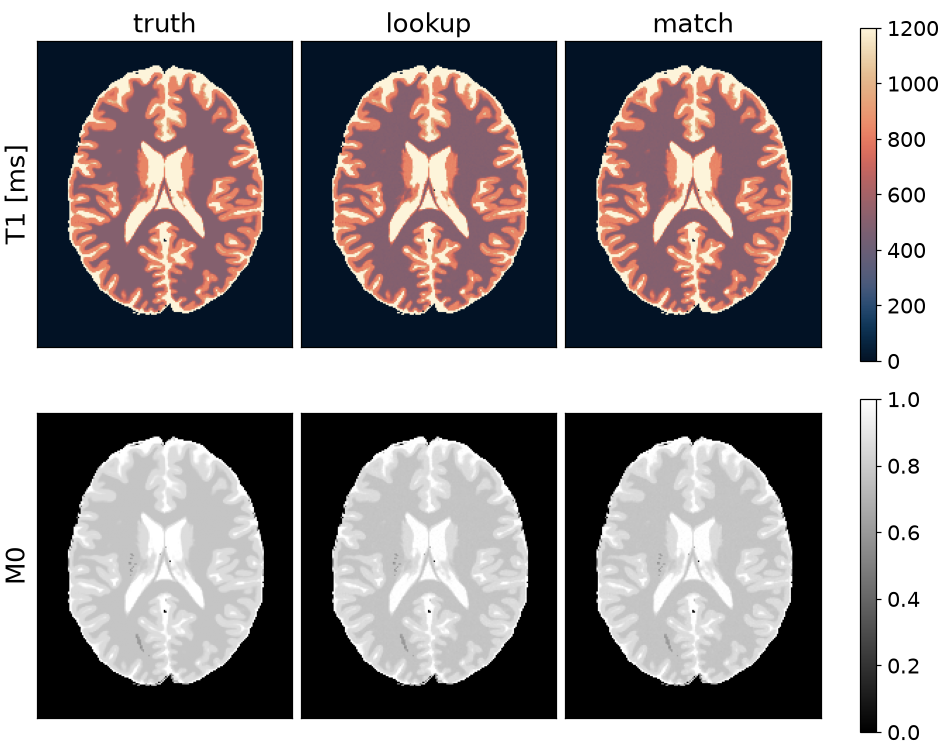
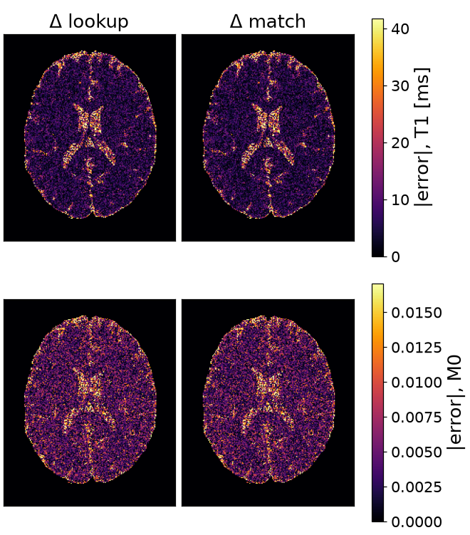
At the point count each needs: the table at sixty, the match at a grid fine enough not to limit it.

the table keeps 38 of 60 points -- the monotonic run -- and spans unified -0.50 to 0.49

Neither estimates M0. Both answer with a T1, and the two blocks it predicts are a shape the measurement is a multiple of, so the multiple is one inner product per voxel.

def proton_density(maps):
    """The scale the measurement is, of the blocks the answer predicts."""
    predicted = simulator.simulate(T1=maps["T1"], M0=1.0)
    return (predicted * measured).sum(-1) / predicted.square().sum(-1).clamp_min(1e-12)


M0_map = proton_density(maps)

method                      train      map     model      peak      T1      M0
------------------------------------------------------------------------------
lookup, 60 points           0.00s    0.4ms  0.00 MiB        --   0.75%   0.46%
match, 2000 atoms           0.00s   46.9ms  0.05 MiB        --   0.71%   0.45%

• 
•