Designing an RF pulse by optimal control

The scope of this notebook is to design the samples of an RF pulse directly, by gradient descent through a Bloch simulation of what they do [1].

A slice-selective pulse is designed for one transmit field. Where B1 varies – by a fifth either way across a body at 3 T – the flip inside the slice varies with it. Here a 90 degree excitation is reshaped so that it stays as close to 90 degrees across that range as its samples allow.

[1]

Conolly S, Nishimura D, Macovski A. Optimal control solutions to the magnetic resonance selective excitation problem. IEEE Trans Med Imaging 1986;5(2):106-115.

import math

import torch

from torchsim import SequenceDesign, compose_spinor

Pulse and slice

The pulse is SAMPLES samples long, and under its slice-select gradient each sample turns a spin at x slice thicknesses from the centre by 2 pi TBW x / SAMPLES about z. Its drive is in radians per sample, so the design is stated without a raster or a gradient amplitude: any pulse of this time-bandwidth product plays it.

The starting point is a Hamming-windowed sinc with the area of a 90 degree flip – a small-tip design, played at a large tip.

SAMPLES, TBW = 128, 4.0
x = torch.linspace(-2.0, 2.0, 161, dtype=torch.float64)
turn = 2 * math.pi * TBW / SAMPLES * x

t = torch.arange(SAMPLES, dtype=torch.float64) - (SAMPLES - 1) / 2
sinc = torch.sinc(TBW * t / SAMPLES) * (
    0.54 + 0.46 * torch.cos(2 * math.pi * t / SAMPLES)
)
start = sinc / sinc.sum() * (math.pi / 2)

Transmit field

Every spin is simulated at five transmit scalings, from 0.8 to 1.2 of nominal. The pulse is one; what it does at each scaling is not.

B1 = torch.tensor([0.8, 0.9, 1.0, 1.1, 1.2], dtype=torch.float64)


def excited(real, imag):
    """``|Mxy|`` after the pulse, from ``+z``: ``(B1, x)``."""
    drive = (real + 1j * imag)[:, None, None] * B1[None, :, None]
    a, b = compose_spinor(drive, turn.expand(len(B1), -1))
    return (2 * a.conj() * b).abs()

The cost

Inside the slice the magnetisation should be all transverse, outside it untouched; the transition band between is left free. A small penalty on the pulse’s energy keeps it from buying flatness with power.

inside = (x.abs() < 0.4).double()
outside = (x.abs() > 0.75).double()


def cost(real, imag):
    transverse = excited(real, imag)
    miss = inside * (transverse - 1.0) ** 2 + outside * transverse**2
    energy = (real**2 + imag**2).sum() / (start**2).sum()
    return miss.sum() / (inside.sum() + outside.sum()) / len(B1) + 1e-4 * energy

Optimized pulse

The real and imaginary parts of every sample are the designed parameters, free of limits: the scanner’s peak B1 would be a Bounded on them.

design = SequenceDesign(
    cost, real=start.clone(), imag=torch.zeros(SAMPLES, dtype=torch.float64)
)
result = design.minimize(iterations=100, learning_rate=2e-4)
real, imag = result.parameters["real"], result.parameters["imag"]

with torch.no_grad():
    before = excited(start, torch.zeros_like(start))
    after = excited(real, imag)

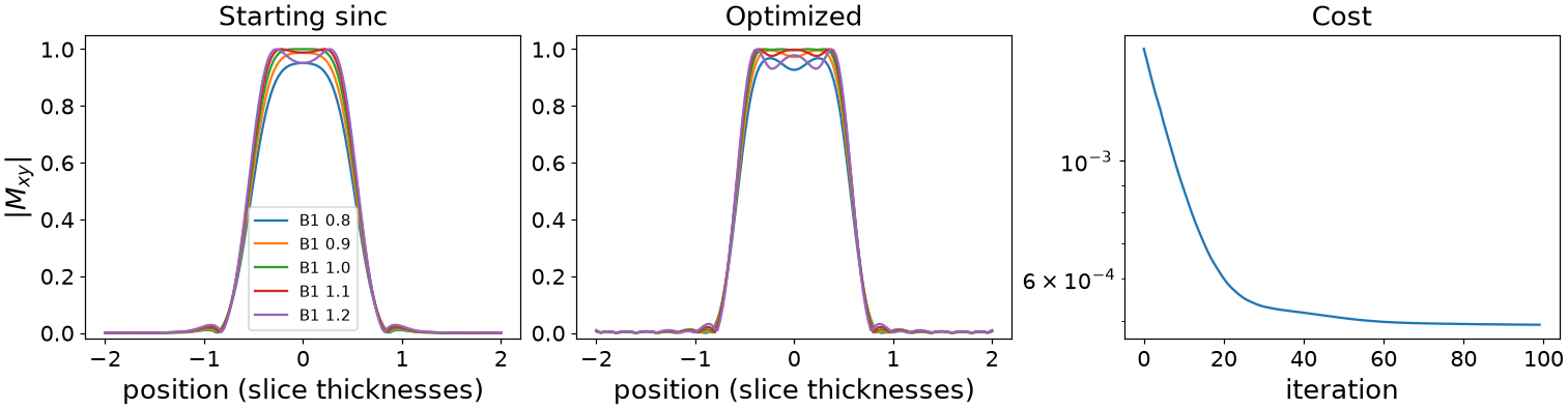
Inside the slice the flip now varies less across the transmit range, most of all where B1 is low, while outside it the leakage stays at the sinc’s level:

centre = inside.bool()
for label, profile in (("starting sinc", before), ("optimized", after)):
    mean = profile[:, centre].mean(dim=1)
    print(
        f"{label:>14}: |Mxy| in the slice at each B1 {[round(float(v), 3) for v in mean]}"
    )

starting sinc: |Mxy| in the slice at each B1 [0.895, 0.94, 0.967, 0.976, 0.969]
    optimized: |Mxy| in the slice at each B1 [0.945, 0.981, 0.996, 0.989, 0.963]