Reconstructing in a linear subspace

The scope of this notebook is to reconstruct one undersampled radial multi-echo spin echo three ways – gridding, conjugate gradients per echo, and a linear subspace – and to report what each costs and gets wrong.

A quantitative scan is usually reconstructed twice: once per contrast, then voxel by voxel into maps. The first step recovers eight images when the answer is two numbers per voxel, each from its own undersampled data. A subspace removes both problems without leaving linear algebra: the signals span far fewer directions than there are contrasts, so reconstructing the coefficients shortens the unknown and ties the echoes together.

The phantom is BrainWeb’s, reached through brainweb-dl: get_mri fetches the fuzzy tissue memberships, and the package ships the table of relaxation times that goes with them – which is what the two standard library imports read.

import csv
from pathlib import Path

import brainweb_dl
from brainweb_dl import get_mri

The Fourier encoding is not TorchSim’s and never will be. mri-nufft supplies the radial trajectory and the non-uniform transform that plays it; deepinv supplies the linear solver a Gauss-Newton step hands its linearized problem to, and the LinearPhysics base class the encoding operator below is written against.

That base class is the whole of the adapter: anything exposing A and A_adjoint composes with what TorchSim supplies, so the operator built a few cells down is the only glue this integration needs.

import mrinufft
from deepinv.optim.linear import least_squares
from deepinv.physics import LinearPhysics
from mrinufft.operators.subspace import MRISubspace
from mrinufft.trajectories import initialize_2D_radial

From TorchSim: the sequence, the estimator the contrast-then-fit routes need, and modes, which hands the temporal basis to mri-nufft in the layout its subspace operator reads.

import time

import numpy as np
import torch

from torchsim.estimators import DictionaryMatcher
from torchsim.simulators import MultiEchoSimulator

What the experiment is: a 96 matrix read as 16 radial spokes per echo, eight echoes, and the rank the temporal basis is fitted at.

SIZE = 96
ECHOES = 8
SPOKES = 16
SAMPLES = 192
RANK = 3

# deepinv's ``gamma`` is the *inverse* regularization weight: it minimizes
# ``||Ax - y||^2 + (1/gamma)||x||^2``, so a smaller number regularizes harder.
# Each route below was given the best of a short sweep -- a few lines, not
# shown -- so what the table compares is routes rather than tuning effort.
CONTRAST_GAMMA = 0.01
SUBSPACE_GAMMA = 10.0

# The GPU transform is used when it is both installed and usable; the
# simulation follows it, so the images and the operator meet on one device.
on_gpu = torch.cuda.is_available() and mrinufft.check_backend("cufinufft")
device = "cuda" if on_gpu else "cpu"
backend = "cufinufft" if on_gpu else "finufft"

Phantom

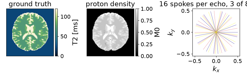
BrainWeb subject 0, slice 90, resampled to the matrix reconstructed here. BrainWeb publishes fuzzy memberships rather than labels, so weighting the tabulated relaxation times by them gives a T2 map whose mixed voxels sit between the pure ones, known everywhere.

Sequence and sampling

A multi-echo spin echo on a golden-angle radial trajectory that rotates between echoes. Sixteen spokes per echo across a 96-sample matrix is roughly ninefold undersampled, which is where the routes disagree.

TE = torch.linspace(10.0, 150.0, ECHOES)
simulator = MultiEchoSimulator(TE=TE)

images = (
    torch.as_tensor(simulator.to(device).simulate(T2=T2_true)).to(torch.complex64)
    * M0_true.to(torch.complex64)[..., None]
)

trajectory = (
    initialize_2D_radial(SPOKES * ECHOES, SAMPLES, tilt="golden")
    .astype(np.float32)
    .reshape(ECHOES, SPOKES * SAMPLES, 2)
)

build = mrinufft.get_operator(backend)
per_echo = [
    build(trajectory[echo], (SIZE, SIZE), n_coils=1, squeeze_dims=False, density=True)
    for echo in range(ECHOES)
]


class RadialEncoding(LinearPhysics):
    """``(batch, echoes, x, y)`` images to k-space, one trajectory per echo.

    This is the whole of ``P F C`` for this experiment, and none of it is
    TorchSim's: it wraps mri-nufft, which is what a real pipeline would do
    with its own trajectory, its own density compensation and its own coils.
    """

    def A(self, x, **kwargs):
        return torch.stack(
            [per_echo[e].op(x[:, e][:, None])[:, 0] for e in range(ECHOES)], 1
        )

    def A_adjoint(self, y, **kwargs):
        return torch.stack(
            [per_echo[e].adj_op(y[:, e][:, None])[:, 0] for e in range(ECHOES)], 1
        )


encoding = RadialEncoding()
kspace = encoding.A(images.movedim(-1, 0)[None])

# The k-space is scaled so the adjoint image peaks at one. Every damping
# weight below is then a number about the model rather than about the
# receiver gain, which is what makes one choice of it transferable.
gridded = encoding.A_adjoint(kspace)[0].movedim(0, -1)
scale = float(gridded.abs().max())
kspace, gridded = kspace / scale, gridded / scale

16 spokes per echo: 9x undersampled

The maps on the left are what every route recovers; the spokes on the right are all that is measured of them, one echo’s worth, rotated by the golden angle from the echo before, so the echoes together cover k-space more evenly than any one does.

Estimator and subspace basis

One DictionaryMatcher states the problem and serves every route. Asking it for a rank fits a temporal basis to the training signals; that basis is what the subspace reconstruction is given, and the coefficients it returns come back to the same mapping. Three directions hold essentially all of an eight-echo exponential, read off the basis rather than assumed.

grid = torch.linspace(20.0, 400.0, 500)
mapping = DictionaryMatcher(simulator).fit(T2=grid, M0=1.0, rank=RANK, seed=0)

rank 3 of 8 contrasts keeps 0.999992

Contrast-by-contrast reconstruction

The conventional pipeline in its two usual forms. Gridding is the adjoint with a density weighting: one pass, smooth, biased. Iterating instead solves each echo’s own least-squares problem, as CG-SENSE does. Both are given the same estimator afterwards, so what is compared is the reconstruction.

adjoint = mapping(gridded)["T2"]

images = least_squares(
    A=encoding.A,
    AT=encoding.A_adjoint,
    y=kspace,
    gamma=CONTRAST_GAMMA,
    solver="CG",
    max_iter=40,
)
separate = mapping(images[0].movedim(0, -1))["T2"]

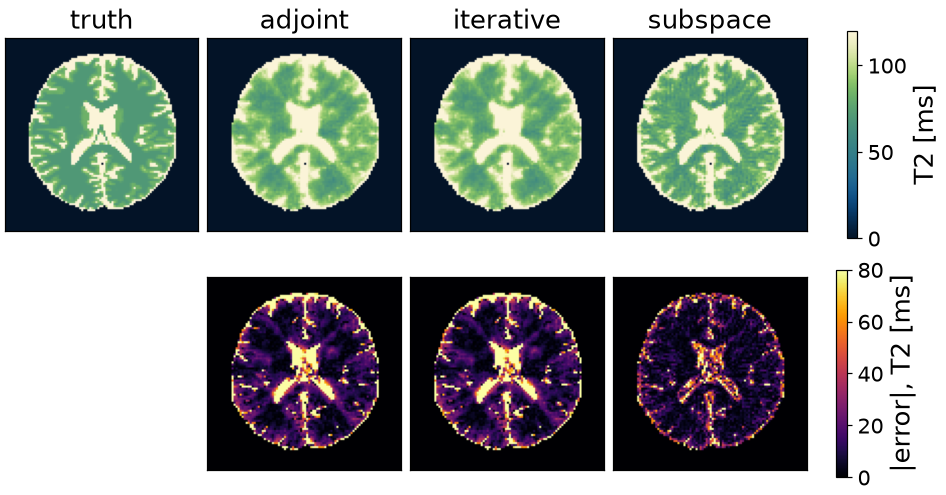
adjoint per echo             0.0s   T2 error  30.6 ms (20.6%)
iterative per echo           0.1s   T2 error  30.7 ms (20.6%)

tensor([[ 52.7455,  61.8838,  58.0762,  ...,  96.9138,  74.0681,  63.4068],
        [ 47.4148,  49.6994,  50.4609,  ...,  91.5832,  66.4529,  77.8758],
        [ 52.7455,  60.3607,  74.0681,  ...,  76.3527,  71.0220,  78.6373],
        ...,
        [ 71.0220,  80.1603, 105.2906,  ...,  74.0681,  51.9840,  64.1683],
        [103.0060, 122.8056, 128.1363,  ...,  93.1062,  64.9299,  56.5531],
        [122.0441, 109.0982, 111.3828,  ...,  82.4449,  82.4449,  69.4990]])

Iterating gains nothing here. Sixteen spokes of 192 samples is 3072 measurements against 9216 unknowns, so each echo alone is underdetermined and there is nothing to converge to that the density-weighted adjoint has not found. Accuracy comes from a constraint across the echoes.

Subspace reconstruction

The signal is written in the basis fitted above and three coefficients are reconstructed instead of eight images. The echoes now constrain one another and the problem is 3072 measurements against 3456 unknowns. It stays linear, so there are no local minima and no starting guess.

mapping.subspace.modes hands the basis over in the layout mri-nufft’s subspace operator reads, and from_coefficients takes what comes back without projecting a second time. The solver is the one the first route used, on a different operator, and one operator now serves every echo.

flat = build(
    trajectory.reshape(-1, 2), (SIZE, SIZE), n_coils=1, squeeze_dims=False, density=True
)
projected = MRISubspace(flat, mapping.subspace.modes.to(device))
projected.n_batchs, projected.n_coils = 1, 1

coefficients = least_squares(
    A=projected.op,
    AT=projected.adj_op,
    y=kspace[:, :, None, :],
    gamma=SUBSPACE_GAMMA,
    solver="CG",
    max_iter=40,
)
linear = mapping.from_coefficients(coefficients[0][:, 0].movedim(0, -1))["T2"]

iterative subspace           0.3s   T2 error  16.9 ms (13.1%)

tensor([[ 51.9840,  73.3066,  67.2144,  ...,  86.2525,  60.3607,  35.2305],
        [ 20.0000,  23.0461,  30.6613,  ..., 102.2445,  41.3226,  70.2605],
        [ 30.6613,  66.4529, 121.2826,  ...,  64.1683,  65.6914,  71.7836],
        ...,
        [ 33.7074,  20.0000, 105.2906,  ...,  76.3527,  50.4609,  81.6834],
        [ 82.4449, 160.8818, 157.0742,  ..., 110.6212,  50.4609,  38.2766],
        [ 93.1062,  84.7295, 110.6212,  ..., 115.9519, 205.0501, 119.7595]])

Maps

The subspace is the only route that constrains the echoes against one another, and it lands at about half the error of either per-contrast route, in a fraction of the time.

Limits

Eight echoes of a single exponential is the case a subspace is best at: three directions hold essentially all of the signal.

Two things break that. A phase-modulated signal – a balanced steady state through a field map, a fingerprinting train with varying RF phase – needs tens of components, and the coefficient problem stops being smaller than the image problem. A model with several parameters has no small basis at all, because the basis must span the product of the ranges. Both cases put the model inside the operator, which is the nonlinear route.

The rank is not a guess: retained says what a basis keeps before anything is projected through it.