3. Custom signal model

Lessons 1 and 2 used shipped simulators. This lesson implements a new one, saturation recovery, by subclassing Simulator. The resulting class supports the same features as a shipped simulator: batched tissue inputs, derivatives with respect to tissue and sequence parameters, and the additional physics of lesson 2.

Learning objectives

• Define the handlers, which map each kind of event to an operator.

• Define the layout, the ordered events of one repetition.

• Validate the model against its closed-form solution.

• Inspect the generated sequence description.

• Differentiate with respect to tissue and sequence parameters.

Previous: 2. Advanced physics. Next: 4. Description-based simulation, where the events are read from a Pulseq file or a scanner instead of the layout.

Sequence

Each block of the sequence is a 90-degree pulse followed by a spoiler, which nulls the magnetization; a saturation time TS of free recovery; and a low-flip-angle spoiled readout. Over a set of saturation times the signal is

\[S(T_S) = M_0 \sin\alpha \, \left(1 - e^{-T_S/T_1}\right).\]

which serves as the reference for the simulation.

Handlers

A sequence consists of RF, ADC and wait events. The handlers define the operator that plays each kind of event. They are class attributes of the simulator, one per kind: excitation, refocusing, inversion, saturation, readout and delay (free precession with no RF and no ADC). Unset handlers keep their defaults.

Saturation recovery uses four. The saturation handler is a 90-degree pulse composed with a spoiler through @. The readout is SPGRReadout(), a sample followed by ideal transverse spoiling:

import torch

from blochsim import Delay, Excitation, SPGRReadout, Spoil
from blochsim import Simulator


def Saturate(flip_rad=torch.pi / 2, phase_rad=0.0):
    """A 90-degree pulse, then a spoiler."""
    return Excitation(flip_rad, phase_rad) @ Spoil()


class SaturationRecovery(Simulator):
    saturation = Saturate  # plays a saturation pulse
    excitation = Excitation  # plays an excitation pulse
    delay = Delay  # plays a wait
    readout = SPGRReadout  # plays a readout, then spoils
    states = 1

Since every block starts and ends with spoiling, no transverse coherence survives between blocks, and a single configuration state (states = 1) is exact.

The handlers also determine how an external description is simulated. A Pulseq file or a scanner stream specifies RF pulses, ADC windows and timing, but blochsim does not take gradients from it. When such a description is simulated (lesson 4), the handlers define the dephasing between events: spoiled, unbalanced or balanced.

Layout

The layout returns the events of one repetition in playing order, built from the handlers through self.operators. It is the default sequence description, generated by the constructor from the sequence parameters. Timestamps are derived from the duration of each operator.

The sequence parameters are the keyword arguments of layout: here the saturation times in milliseconds and the readout flip angle in degrees. Operators take SI units (seconds, radians).

class SaturationRecovery(SaturationRecovery):
    def layout(self, *, TS, flip):
        angle = torch.deg2rad(torch.as_tensor(flip))
        parts = []
        for wait in torch.as_tensor(TS) * 1e-3:  # ms to s
            parts += [self.operators.saturation(), self.operators.delay(wait)]
            parts += [self.operators.excitation(angle), self.operators.readout()]
        return parts

Simulation

The class is used like a shipped simulator:

TS = torch.logspace(1.3, 3.7, 40)  # 20 ms to 5 s
T1 = torch.tensor([830.0, 1330.0, 4000.0])

recovery = SaturationRecovery(TS=TS, flip=10.0)
signal = recovery.simulate(T1=T1, T2=torch.tensor([80.0, 110.0, 2000.0]))

closed_form = torch.sin(torch.deg2rad(torch.tensor(10.0))) * (
    1 - torch.exp(-TS / T1[:, None])
)
print(f"largest difference: {(signal.abs() - closed_form).abs().max():.1e}")

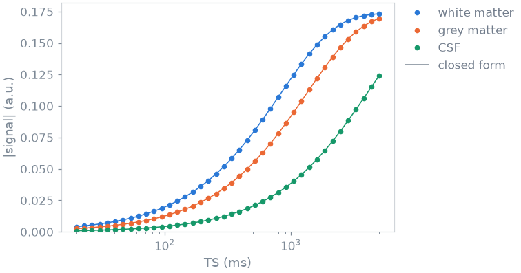
largest difference: 3.0e-08

The simulation matches the closed form to single precision. Since blochsim evaluates the events individually, the agreement validates the layout.

Sequence description

describe returns the events your layout produced, with their timestamps, as a SequenceDescription; plot displays them. This is the first thing to inspect when a result is unexpected:

description = recovery.describe(TS=[50.0, 100.0, 200.0], flip=10.0)

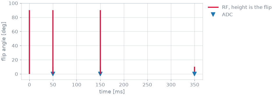
Three blocks, each with a saturation pulse, a wait of increasing length, a 10-degree excitation and a readout. Lesson 4 reads the same kind of object from a Pulseq file or a scanner.

Derivatives

jacobian works on the new class without additional code. The derivative with respect to T1 is what a T1 fit requires:

signal, dT1 = recovery.jacobian("T1", T1=T1, T2=80.0)

Sequence parameters are PyTorch tensors, so derivatives with respect to them are obtained by reverse-mode autodiff (backward). Here, the gradient of the summed signal with respect to each saturation time:

TS_designed = TS.clone().requires_grad_(True)
total = recovery.simulate(TS=TS_designed, T1=830.0, T2=80.0).abs().sum()
total.backward()

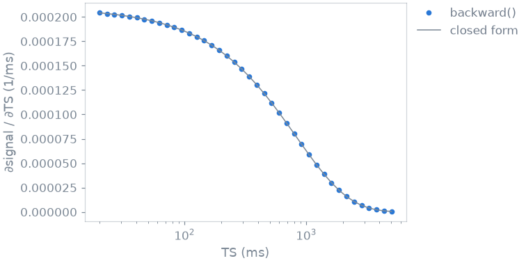
This gradient is the basis of sequence optimization; the sequence design Applications use it on complete protocols.

Additional physics

The physics of lesson 2 is controlled by tissue properties and therefore applies to the new class unchanged. With B1 = 0.8 the saturation pulse is 72 degrees, and saturation is incomplete:

low_b1 = recovery.simulate(T1=830.0, T2=80.0, B1=0.8)
ideal = recovery.simulate(T1=830.0, T2=80.0)

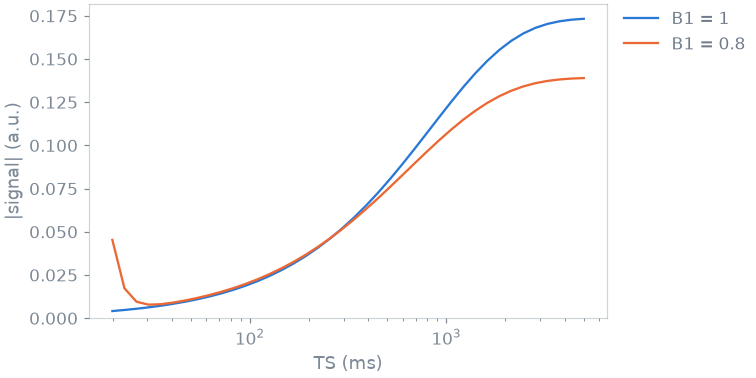
At short saturation times the residual longitudinal magnetization raises the signal; at long ones the 8-degree readout lowers it. A T1 fit that ignores B1 is biased by both effects.

Specification

What this lesson built, stated the way you would ask an agent for it:

Write a blochsim Simulator for saturation recovery. Handlers: a saturation
that is a 90-degree pulse followed by a spoiler, an ideal excitation, a
delay, and a spoiled readout; keep one configuration state. The layout
takes the saturation times TS (ms) and the readout flip angle (deg), and
plays saturate, wait TS, excite, read for each TS. Check it against
M0 sin(flip) (1 - exp(-TS/T1)) in white matter, grey matter and CSF.