5. Testing on the virtual scanner

This lesson is optional: it extends the course rather than completing it. The virtual scanner stands in for the scanner and nothing else, so a sequence and a reconstruction plugin can be tested before a scanner is involved. It acquires in two ways: along the played trajectory from an analytic phantom, which leaves relaxation out, or by a Bloch simulation of every block the cache plays. The conversion itself is checked by comparing the gradients a sequence asks for with those its cache plays. The models are described in The virtual scanner.

Learning objectives

• Acquire a phantom with acquire() and simulate it on isochromats with simulate(), and state what each models.

• Check a cache against the sequence it was converted from with validate().

The previous lesson reconstructed a series with a plugin of its own.

A sequence with T1 contrast

The design is the 2D gradient echo at a 20 ms TR and a 30° flip angle, without dummy scans, converted into its cache. The phantom holds two ellipses of equal proton density and T2, with a T1 of 300 ms on the left and 1500 ms on the right.

import tempfile
from pathlib import Path

import numpy as np
import pypulseqpp as pp
from pypulseqpp.sequences.sequence.gre2D_sequence import gre2d

from pulserver import ir, virtual
from pulserver.proxy import SequenceTable

system = pp.Opts(max_grad=40, grad_unit="mT/m", max_slew=150, slew_unit="T/m/s")
path = Path(tempfile.mkdtemp()) / "gre2d.seq"
gre2d(system, n_x=64, n_y=64, tr=0.02, flip_angle_deg=30.0, n_dummy=0).write(path)
ir.convert(path, system)

phantom = virtual.Phantom(
    [
        virtual.Ellipse((-0.04, 0.0, 0.0), (0.03, 0.05), t1=0.3, t2=0.08),
        virtual.Ellipse((0.04, 0.0, 0.0), (0.03, 0.05), t1=1.5, t2=0.08),
    ]
)

Two acquisitions

acquire() evaluates the phantom’s analytic transform at the k-space location of every sample: each excitation tips the whole magnetization, whatever the flip angle and T1. The isochromats of isochromats(), here on a 1 mm grid, are played block by block by simulate() with the Bloch equation, so the flip angle, relaxation and the approach to steady state act on the signal.

analytic = virtual.acquire(path, phantom)
simulated = virtual.simulate(path, phantom.isochromats(1e-3))

Both return one array of samples per readout in play order; the encoding counters of the sequence place them in k-space.

lines = SequenceTable.read(path).counters["LIN"]


def image(readouts):
    kspace = np.zeros((64, readouts[0].shape[-1]), complex)
    kspace[lines] = np.stack([readout[0] for readout in readouts])
    pixels = np.fft.fftshift(np.fft.ifft2(np.fft.ifftshift(kspace)))
    return np.abs(pixels[:, 32:96])


images = {"acquire": image(analytic), "simulate": image(simulated)}
inside = images["acquire"] > 0.5 * images["acquire"].max()
short_t1, long_t1 = inside.copy(), inside.copy()
short_t1[:, 32:], long_t1[:, :32] = False, False
for name, pixels in images.items():
    ratio = pixels[short_t1].mean() / pixels[long_t1].mean()
    print(f"{name}: mean signal, short T1 over long T1, {ratio:.2f}")

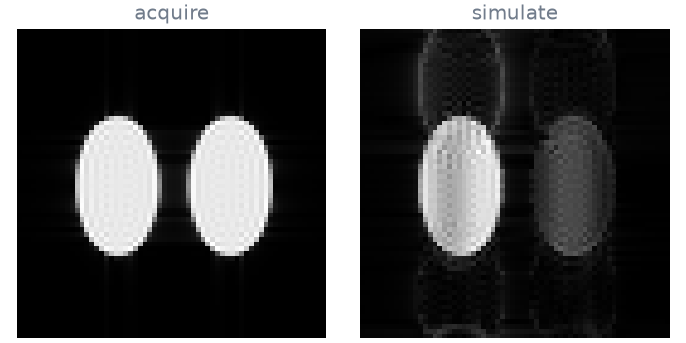
acquire: mean signal, short T1 over long T1, 1.00
simulate: mean signal, short T1 over long T1, 3.28

The analytic acquisition shows two ellipses of equal signal: it tests the trajectory, the encoding and the reconstruction. The Bloch simulation shows the T1 weighting of a spoiled gradient echo at a short TR and, since the scan plays no dummy scans, the ghosts along the phase-encoding axis that the approach to steady state leaves. It tests the sequence’s contrast.

Conversion check

validate() compares the gradients the sequence asks for with a second rendering. Without a recording of a scanner playing it, the rendering is the cache’s own waveforms. Agreement establishes that the conversion kept the sequence; it does not establish that a scanner plays it.

from pulserver.validate import validate

print(validate(path, system=system))

the sequence agrees with the ir waveforms
  gx     largest difference 9.542e-06 of 38.79 (0.00%)
  gy     largest difference 7.34e-08 of 21.35 (0.00%)
  gz     largest difference 3.35e-10 of 35.63 (0.00%)