Field-of-view offset and the proxy phase

This Tour moves the field of view of two designs away from the isocentre and shows where the phase of the offset is applied: by the scanner, as the frequency and phase offsets of each readout, and by the reconstruction proxy, for the part those offsets cannot carry when the readout gradient varies during sampling.

Prerequisites: lessons 3 and 4 of the course.

An object at \(\mathbf{d}\) adds the phase \(-2\pi\,\mathbf{d}\cdot\mathbf{k}(t)\) to each sample. Under a readout gradient that holds one value, \(\mathbf{k}(t)\) is linear in time and the phase is a frequency and a phase offset. On a ramp-sampled readout it is not, and the IR cache carries no ADC phase modulation for the rest (Raw-data enrichment and routing).

Two designs at an offset

A 2D gradient echo, which samples the flat top of its readout gradient, and a 2D echo planar sequence, whose trains are ramp sampled, are converted at the prescribed offset \(\mathbf{d} = (30, -50, 0)\) mm along the logical readout, phase-encoding and slice axes, and again at the isocentre.

import tempfile
from pathlib import Path

import numpy as np
import pypulseqpp as pp
from pypulseqpp import sequences
from pypulseqpp.sequences.sequence.epi2D_sequence import epi2d
from pypulseqpp.sequences.sequence.gre2D_sequence import gre2d

from pulserver import ir, virtual
from pulserver.proxy import SequenceTable

system = pp.Opts(max_grad=40, grad_unit="mT/m", max_slew=150, slew_unit="T/m/s")
work = Path(tempfile.mkdtemp())
offset = (0.03, -0.05, 0.0)

designs = {
    "gradient echo": [gre2d(system, n_x=64, n_y=64, n_dummy=0)],
    "echo planar": epi2d(system, n_x=64, n_y=64),
}
files = {}
for name, chain in designs.items():
    for where, shift in (("offset", offset), ("isocentre", None)):
        path = work / f"{name.replace(' ', '_')}_{where}.seq"
        files[name, where] = sequences.write(path, chain, offline=False)[0]
        ir.convert(files[name, where], system, fov_offset=shift)

Acquisitions

The phantom is acquired twice per design: placed at \(\mathbf{d}\) and played from the cache converted at the offset, and placed at the isocentre and played from the cache converted there. Under the identity rotation the physical axes are the logical ones.

ellipses = [
    virtual.Ellipse((0.0, 0.0, 0.0), (0.06, 0.04)),
    virtual.Ellipse((0.02, 0.01, 0.0), (0.015, 0.015), intensity=-0.5),
]
at_offset = virtual.Phantom(ellipses, position=offset)
at_isocentre = virtual.Phantom(ellipses)

readouts = {
    name: (
        virtual.acquire(files[name, "offset"], at_offset),
        virtual.acquire(files[name, "isocentre"], at_isocentre),
    )
    for name in designs
}

The proxy phase

SequenceTable, read at the offset the cache was converted at, gives the phase the proxy applies to each readout, in rad, or None where the scanner’s offsets carry the whole phase.

tables = {
    name: SequenceTable.read(files[name, "offset"], fov_offset_m=offset)
    for name in designs
}
for name, table in tables.items():
    phases = [table.readout_phase_modulation(row) for row in range(len(table))]
    applied = sum(phase is not None for phase in phases)
    print(f"{name}: a phase on {applied} of {len(table)} readouts")

gradient echo: a phase on 0 of 64 readouts
echo planar: a phase on 134 of 134 readouts

On the echo planar readouts the phase is the curvature of \(2\pi\,\mathbf{d}\cdot\mathbf{k}(t)\) about the line through the middle of the sampling window, which the scanner’s frequency and phase offsets play. The imaging readouts are those of the encoding space of the main subsequence that is not the navigators’.

table = tables["echo planar"]
main = max(index for index, space in enumerate(table.spaces) if not space.navigator)
imaging = np.flatnonzero(table.encoding_space == main)
row = imaging[len(imaging) // 2]

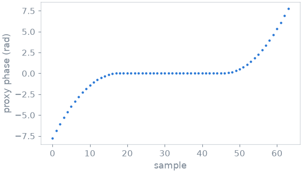
With the proxy phase applied, the samples of the object at the offset are those of the object at the isocentre, to the precision of the acquisition; as received, the echo planar samples are not.

def agreement(name, corrected):
    moved, centred = readouts[name]
    table = tables[name]
    worst = 0.0
    for row in range(len(table)):
        samples = moved[row]
        phase = table.readout_phase_modulation(row)
        if corrected and phase is not None:
            samples = samples * np.exp(1j * phase)
        worst = max(
            worst, np.abs(samples - centred[row]).max() / np.abs(centred[row]).max()
        )
    return worst


for name in designs:
    print(
        f"{name}: largest difference from the isocentre, as received "
        f"{agreement(name, False):.1e}, with the proxy phase {agreement(name, True):.1e}"
    )

gradient echo: largest difference from the isocentre, as received 9.5e-07, with the proxy phase 9.5e-07
echo planar: largest difference from the isocentre, as received 1.1e+00, with the proxy phase 9.4e-07

Images

The echo planar lines are gridded along the readout from the k-space of their samples, placed by their encoding counters, and Fourier transformed. The differences from the image at the isocentre show what the phase the proxy applies removes. The arcs at the sides of the reference come from the linear interpolation of the gridding, which the three images share.

def image(samples, table):
    n, fov = 64, 0.22
    grid = (np.arange(n) - n / 2) / fov
    kspace = np.zeros((n, n), complex)
    for row in imaging:
        kx = table.readout_k(row)[0]
        order = np.argsort(kx)
        line = samples[row][0][order]
        kspace[table.counters["LIN"][row]] = np.interp(
            grid, kx[order], line.real
        ) + 1j * np.interp(grid, kx[order], line.imag)
    return np.abs(np.fft.fftshift(np.fft.ifft2(np.fft.ifftshift(kspace))))


moved, centred = readouts["echo planar"]
reference = image(centred, table)
as_received = image(moved, table)
corrected = image(
    [
        samples
        if table.readout_phase_modulation(row) is None
        else samples * np.exp(1j * table.readout_phase_modulation(row))
        for row, samples in enumerate(moved)
    ],
    table,
)

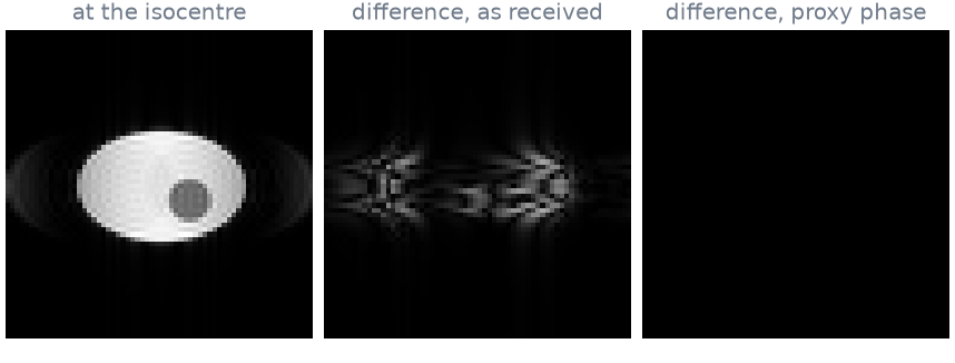
The differences are drawn at a fifth of the reference’s scale. A header that states the object at another position, fov_offset_mm, makes the proxy apply \(2\pi\,\Delta\mathbf{d}\cdot\mathbf{k}(t)\) in full for the difference, as readout_phase_modulation() states, which needs no new cache.