PERK: kernel ridge regression

The scope of this notebook is to map a brain slice with PERK, to show what the size of the regression buys, and to read the error bar it reports.

PERK never builds a dictionary. It is a kernel regression trained on signals drawn from a prior rather than laid on a grid, and at inference it projects a signal onto a fixed set of random Fourier features and reads the answer off a linear combination of them. Its cost per voxel does not depend on how many parameters are unknown, and the training is paid once.

The problem is stated over a simulator carrying the sequence and filled in by an estimator. execution() decides where that work runs, and the timings below are taken inside it.

import time

import numpy as np
import torch

import torchsim
from torchsim import (
    Subspace,
)
from torchsim.estimators import PERK, DictionaryMatcher
from torchsim.simulators import MRFSimulator

Phantom

BrainWeb subject 0, slice 90: an axial slice at 1 mm through the lateral ventricles. BrainWeb publishes fuzzy memberships rather than labels, so each voxel holds a fraction of each tissue, and the relaxation times are weighted by those fractions. A third of the voxels are mixtures, so the truth is a continuum and not four values.

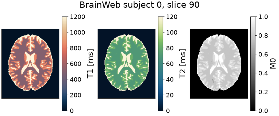
Text(0.5, 0.9883529057497298, 'BrainWeb subject 0, slice 90')

Sequence

Four hundred repetitions after an inversion, at a fixed repetition time and a flip angle that varies smoothly along the train. A schedule that jumped about would give trajectories differing by noise rather than by physics.

CONTRASTS = 400
TR_MS = 10.0
TI_MS = 20.0

repetition = torch.arange(CONTRASTS, dtype=torch.float32)
flip = 10.0 + 50.0 * torch.sin(torch.pi * repetition / CONTRASTS) ** 2

simulator = MRFSimulator(flip=flip, TR=TR_MS, TI=TI_MS, states=20, M0=1.0)

The readouts wind the states on rather than rewinding them, so nothing returns transverse magnetization to the imaginary axis: the trajectory comes back real to within 3e-8, which halves both the dictionary and the arithmetic that searches it.

fingerprints = simulator.simulate(
    T1=torch.tensor([500.0, 833.0, 2569.0]), T2=torch.tensor([70.0, 83.0, 329.0])
).real

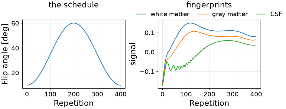
[<matplotlib.legend.Legend object at 0x7f1b8c451130>]

The measurement, with noise at 2% of the peak fingerprint. One number sets it, and the same number is what the estimators are told to expect – an estimator trained for more noise than the scan has learns to distrust the data and answers with the prior instead.

NOISE_STD = float(0.02 * fingerprints.max())

truth = {
    "T1": torch.as_tensor(T1_true[mask].copy()),
    "T2": torch.as_tensor(T2_true[mask].copy()),
}
density = torch.as_tensor(M0_true[mask].copy())
clean = simulator.simulate(**truth).real * density[:, None]
generator = torch.Generator().manual_seed(42)
measured = clean + NOISE_STD * torch.randn(clean.shape, generator=generator)

Problem statement

What is unknown, over what range, and at what noise level. Both relaxation times span more than a decade, so the prior is drawn logarithmically: uniform sampling would spend most of the budget on long T1, where the trajectories are nearly parallel.

T1_RANGE = (200.0, 5000.0)
T2_RANGE = (20.0, 600.0)
SAMPLES = 20_000
prior = torch.Generator().manual_seed(11)

Subspace basis

Four hundred contrasts do not span four hundred directions. A basis fitted to simulated trajectories says how many they do span; one minus the energy it keeps is the relative squared error of projecting through it and back.

training_signals, _, _ = (
    PERK(simulator)
    .fit(
        T1=log_uniform(*T1_RANGE, SAMPLES),
        T2=log_uniform(*T2_RANGE, SAMPLES),
        noise_std=NOISE_STD,
        seed=0,
    )
    .training_set(SAMPLES)
)
training_signals = training_signals.real

RANK = 4

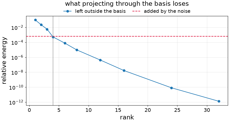
[<matplotlib.legend.Legend object at 0x7f1b8ddde120>]

Four directions leave less outside the basis than the noise puts in, so rank 4 is used from here on.

Training

Twenty thousand parameter pairs drawn from the prior, simulated, and given the noise the scan has. Fitting is a linear solve against the features.

FEATURES = 1000

perk = PERK(simulator, n_features=FEATURES, regularization=1e-6, normalize=True).fit(
    T1=log_uniform(*T1_RANGE, SAMPLES),
    T2=log_uniform(*T2_RANGE, SAMPLES),
    noise_std=NOISE_STD,
    seed=0,
    rank=RANK,
    samples=SAMPLES,
)

maps = perk(measured)  # {"T1": ..., "T2": ...}, one value per voxel

dictionary: 20000 atoms at rank 4; regression: 1000 features from 20000 training draws

Cost and accuracy

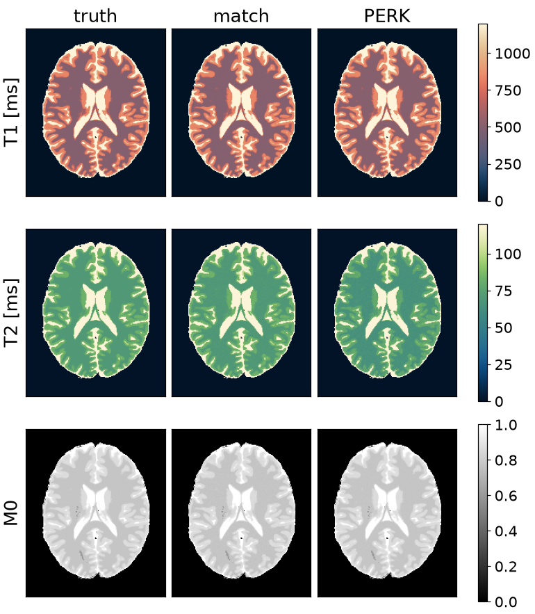
Best of three passes each, after a warm-up. model is what the fitted estimator carries between volumes; peak is the high-water mark on the card while the slice was mapped, and a dash on a machine with no card. The dictionary row is the reference point.

method                       train     map     model      peak      T1      T2
------------------------------------------------------------------------------
match, rank 4                 1.0s   1.54s   1.4 MiB        --    0.6%    1.6%
PERK, 500 features            1.2s   0.03s   0.0 MiB        --    0.9%   13.2%
PERK, 1000 features           1.6s   0.04s   0.1 MiB        --    1.3%    5.7%
PERK, 4000 features           8.6s   0.10s   0.4 MiB        --    0.9%    5.5%

Maps

• 
• 

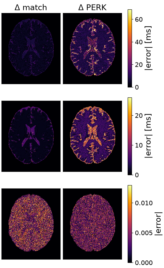
Uncertainty

uncertainty=True returns a second set of maps: how far the answer is expected to sit from the truth. PERK learns that at training, from the residuals of its own fit, so reporting it is a matrix multiply rather than a rerun of the volume.

maps, spread = perk(measured, uncertainty=True)

Read against the Cramer-Rao bound, the lowest standard deviation an unbiased estimate could reach from this train at this noise. The bound belongs to the sequence, so the gap is what the method loses.

_signal, sensitivity = simulator.jacobian("T1 T2".split(), **truth)
sensitivity = sensitivity.real * density[:, None, None]
floor = torchsim.crlb(sensitivity, noise_variance=NOISE_STD**2, singular="infinite")
bound = {"T1": floor[:, 0].sqrt(), "T2": floor[:, 1].sqrt()}

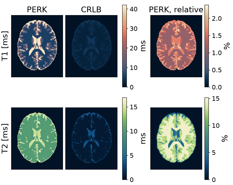
            PERK      CRLB     PERK   (median over the brain)
T1        8.4 ms    2.4 ms     1.2%
T2       10.2 ms    0.5 ms    12.8%

Each row uses its own parameter’s colormap. The two absolute panels share a scale; the third is the same spread as a percentage of the relaxation time, which is what says whether ten milliseconds is tight.

Both are largest in CSF, whose long T1 this train resolves least. The gap between them is not: T1 sits within a small multiple of the bound, T2 several times above it, and it is T2 whose error moved when the feature count was swept. One is a sequence to redesign, the other a regression to enlarge.

The number is not the noise alone. A regression trained on a prior answers with the prior where the data is weak, and is wrong the same way in every realization, so repeating the scan would never show that part.