Free induction decay

The smallest complete Pulseq sequence is a pulse-acquire experiment: one excitation pulse followed by one acquisition window. This first lesson of the course builds it and introduces the objects every later lesson extends: the system limits against which a factory designs an event, the RF and ADC events, the blocks in which events are played, the timing check, and the .seq file. A Bloch simulation of the stored pulse relates the transverse magnetisation to the flip angle.

The representation these objects belong to is described in Events and blocks.

Learning objectives

After this lesson, you should be able to:

• define system limits, rasters and dead times;

• create a hard RF pulse and an ADC event, and relate the number of samples, the dwell time and the receiver bandwidth;

• place events in blocks and set a repetition time with a delay;

• read a pulse-sequence diagram of the result;

• check the sequence timing and write the sequence to a .seq file.

System limits

Every factory solves its waveforms against a set of limits, and every event time is quantized to the rasters those limits declare. The dead times bound what the transmit and receive chains can do rather than what the sequencer can address, and the timing check reports them separately.

import numpy as np

import pypulseqpp as pp

system = pp.Opts(
    max_grad=32.0,
    grad_unit="mT/m",
    max_slew=130.0,
    slew_unit="T/m/s",
    rf_dead_time=100e-6,
    rf_ringdown_time=20e-6,
    adc_dead_time=10e-6,
)

Two events

A rectangular pulse of constant amplitude, and an acquisition window of 8192 samples. The dwell time is the sampling interval, and its reciprocal is the receiver bandwidth; calc_adc_timing() moves a requested dwell onto the ADC raster and lands the acquisition duration on the gradient raster. The timing check requires both.

FLIP_ANGLES_DEG = (10.0, 30.0, 60.0, 90.0)

pulses = [
    pp.make_block_pulse(
        flip_angle=np.deg2rad(flip_angle),
        duration=200e-6,
        delay=system.rf_dead_time,
        system=system,
        use="excitation",
    )
    for flip_angle in FLIP_ANGLES_DEG
]
dwell, acquisition = pp.calc_adc_timing(
    8192,
    32e-6,
    grad_raster_time=system.grad_raster_time,
    adc_raster_time=system.adc_raster_time,
)
adc = pp.make_adc(
    num_samples=8192, dwell=dwell, delay=system.adc_dead_time, system=system
)

print(
    f"dwell {dwell * 1e6:.0f} us, receiver bandwidth {1e-3 / dwell:.1f} kHz, "
    f"acquisition {acquisition * 1e3:.1f} ms"
)

dwell 40 us, receiver bandwidth 25.0 kHz, acquisition 327.7 ms

Two blocks

A block holds at most one event per channel, and the events in it start together on the block’s clock. Blocks are played back to back, so the acquisition begins when the pulse’s block ends.

One repetition per flip angle. A block lasts as long as its longest event, so a delay event longer than the acquisition window in the acquisition block sets the repetition time.

seq = pp.Sequence(system=system)
for pulse in pulses:
    seq.add_block(pulse)
    seq.add_block(adc, pp.make_delay(500e-3))

ok, errors = seq.check_timing()
print(f"timing {ok}, {seq.num_blocks} blocks, {seq.duration()[0]:.2f} s")

timing True, 8 blocks, 2.00 s

Sequence diagram

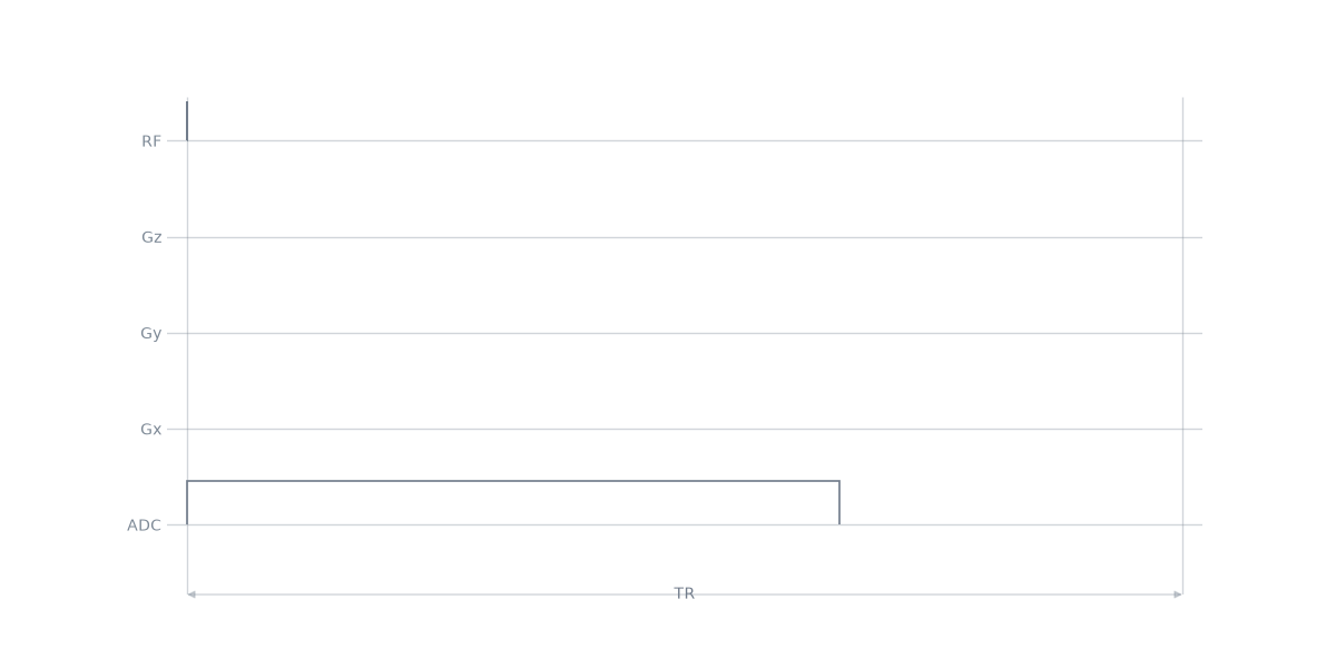
The solid trace is one repetition; the shaded traces are the others, which differ only in the amplitude of the pulse.

seq.paper_plot()

Transverse magnetisation against flip angle

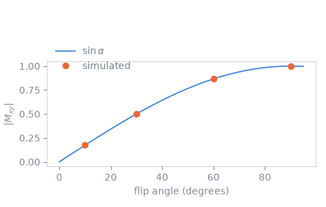
sim_rf() integrates the Bloch equations over the pulse the sequence holds. On resonance a rectangular pulse rotates the magnetisation by its nominal flip angle, so the transverse component follows \(|M_{xy}| = \sin\alpha\).

on_resonance = []
for pulse in pulses:
    mz_xy, frequency = pp.sim_rf(pulse)[1:3]
    on_resonance.append(abs(mz_xy[int(np.argmin(abs(frequency)))]))

Writing the file

The definitions are written beside the block table and are what a reconstruction reads to interpret the acquisition.

from pathlib import Path
from tempfile import mkdtemp

seq.set_definition("Name", "fid")
path = Path(mkdtemp()) / "fid.seq"
seq.write(str(path))
print(path.read_text().splitlines()[0])

# Pulseq sequence file