Excitation modules

The earlier sections built slice-selective excitations by hand with a pulse factory. This lesson designs them with the excitation module, and measures how the three numbers that specify a selective pulse — flip angle, slice thickness and time-bandwidth product — affect the slice profile, the selection gradient and the peak \(B_1\), and which combinations of them the gradient system permits.

A slice-selective pulse and its selection gradient are not independent: the gradient has to place the pulse’s bandwidth across the slice,

\[G = \frac{\mathrm{TBW}}{\gamma\, T\, \Delta z} ,\]

so a shorter pulse at the same thickness and the same time-bandwidth product needs a proportionally stronger selection gradient and a proportionally larger \(B_1\). The gradient amplitude limit therefore bounds the two together.

The measured quantities are the simulated slice profile — its transition width and the ripple on either side of it — and the boundary in the duration/time-bandwidth plane beyond which the module raises an error. The module concept, and the reason the design is divided in this way, are described in Sequence modules.

Learning objectives

After this lesson, you should be able to:

• design a slice-selective excitation with the excitation module and simulate its slice profile;

• measure the transition width and the passband and stopband ripple of a profile;

• relate the time-bandwidth product and the pulse duration to the profile, the selection gradient amplitude and the peak \(B_1\);

• identify the designs the gradient amplitude limit permits.

import numpy as np

import pypulseqpp as pp
import pypulseqpp.sequences as design

#: Gyromagnetic ratio of the proton (Hz/T).
GAMMA = 42.576e6

THICKNESS = 5e-3
FLIP_ANGLE_DEG = 8.0

system = pp.Opts(
    max_grad=32.0,
    grad_unit="mT/m",
    max_slew=130.0,
    slew_unit="T/m/s",
    adc_dead_time=10e-6,
)

Simulating a design

The excitation module designs the pulse, its selection gradient and the rephaser that unwinds the second half of the selection. Its sim_rf simulates the Bloch response of its pulse across off-resonance, which under a selection gradient of amplitude selection_amplitude is the slice profile, because a spin at position z is off-resonance by selection_amplitude * z.

def simulate(time_bw_product, duration_s):
    """Design one excitation and simulate the profile its pulse produces."""
    module = design.SpatialSelectiveExcitation(
        system,
        flip_angle_deg=FLIP_ANGLE_DEG,
        thickness_m=THICKNESS,
        duration_s=duration_s,
        time_bw_product=time_bw_product,
    )
    magnetisation, frequency = module.sim_rf()[1:3]
    profile = np.abs(magnetisation)
    return {
        "tbw": time_bw_product,
        "duration": duration_s,
        "gradient": module.selection_amplitude / GAMMA,
        "position": frequency / module.selection_amplitude,
        "profile": profile / profile.max(),
        "time": np.arange(module.rf.signal.size) * system.rf_raster_time,
        "envelope": np.abs(module.rf.signal),
        "peak_b1": float(np.abs(module.rf.signal).max()),
    }

Two numbers describe a profile: how far it takes to fall from the passband to the stopband, and how flat it is on either side of that transition.

def describe(simulated):
    """Transition width, passband ripple and stopband level of a profile."""
    position, profile = simulated["position"], simulated["profile"]
    edge = position > 0
    outward, falling = position[edge], profile[edge]

    def crosses(level):
        index = int(np.argmax(falling < level))
        return np.interp(
            level,
            [falling[index], falling[index - 1]],
            [outward[index], outward[index - 1]],
        )

    passband = profile[np.abs(position) < 0.35 * THICKNESS]
    stopband = profile[np.abs(position) > 1.5 * THICKNESS]
    return {
        **simulated,
        "transition": crosses(0.1) - crosses(0.9),
        "passband": float(passband.max() - passband.min()),
        "stopband": float(stopband.max()),
    }

The time-bandwidth product at a fixed duration

Every design below is 3 ms long and selects the same 5 mm. The pulse has more zero crossings as the time-bandwidth product rises, and the selection gradient rises with it so that the wider bandwidth still lands on the same slice.

PRODUCTS = (2.0, 4.0, 6.0, 8.0, 12.0)

by_product = [describe(simulate(product, 3e-3)) for product in PRODUCTS]

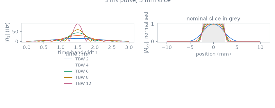
 tbw      gradient    transition    passband    stopband     peak B1
 2.0       3.13 mT/m      3.125 mm      0.2889      0.0041     14.7 Hz
 4.0       6.26 mT/m      1.762 mm      0.1654      0.0022     29.2 Hz
 6.0       9.39 mT/m      1.208 mm      0.0604      0.0014     43.5 Hz
 8.0      12.53 mT/m      0.916 mm      0.0201      0.0010     59.1 Hz
12.0      18.79 mT/m      0.615 mm      0.0143      0.0006     89.0 Hz

Above the smallest product the transition width falls close to inversely with it, so their product settles towards a figure set by the slice thickness rather than by the design. The passband ripple falls over the same range and the stopband stays below a percent throughout. The last column gives the corresponding increase in transmit amplitude: the peak \(B_1\) rises in proportion to the time-bandwidth product, because the same flip angle is delivered by an envelope with more structure in the same time.

The duration at a fixed time-bandwidth product

Varying duration at fixed time-bandwidth product separates slice-profile properties from gradient amplitude and peak \(B_1\) requirements.

DURATIONS = (1e-3, 2e-3, 3e-3, 5e-3, 8e-3)

by_duration = [describe(simulate(4.0, duration)) for duration in DURATIONS]

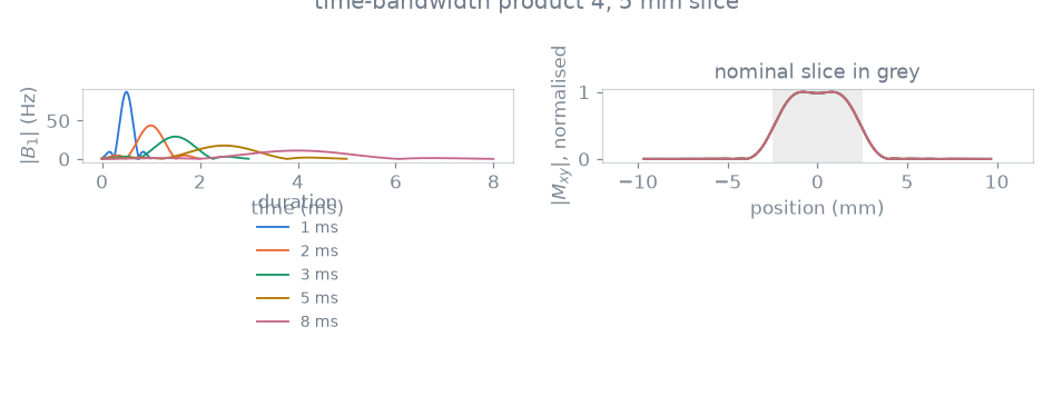
duration_ms      gradient    transition    passband    stopband     peak B1
       1.0      18.79 mT/m      1.761 mm      0.1686      0.0022     87.5 Hz
       2.0       9.39 mT/m      1.762 mm      0.1654      0.0022     43.8 Hz
       3.0       6.26 mT/m      1.762 mm      0.1654      0.0022     29.2 Hz
       5.0       3.76 mT/m      1.762 mm      0.1604      0.0022     17.5 Hz
       8.0       2.35 mT/m      1.763 mm      0.1591      0.0022     10.9 Hz

The five profiles lie on top of each other. The transition width is the same to three decimal places across an eightfold change of duration, and the small residual differences in the ripple follow the number of samples the pulse is written with: on a fixed RF raster a 1 ms envelope has an eighth of the samples of an 8 ms one. The duration sets the selection gradient and the peak \(B_1\), both of which scale as its reciprocal, and the time the repetition spends on the excitation.

Designs admitted by the gradient amplitude limit

The two sweeps are two lines through one plane, and the amplitude limit cuts it along \(T = \mathrm{TBW} / (\gamma\, \Delta z\, G_\mathrm{max})\). A design above that line is realizable; one below it requires a selection gradient above the amplitude limit, and the module raises an error rather than widening the slice.

grid = []
for product in (2.0, 4.0, 6.0, 8.0, 12.0, 16.0):
    for duration in (0.3e-3, 0.5e-3, 1e-3, 2e-3, 3e-3, 5e-3):
        try:
            design.SpatialSelectiveExcitation(
                system,
                flip_angle_deg=FLIP_ANGLE_DEG,
                thickness_m=THICKNESS,
                duration_s=duration,
                time_bw_product=product,
            )
        except ValueError:
            feasible = False
        else:
            feasible = True
        grid.append({"tbw": product, "duration": duration, "feasible": feasible})

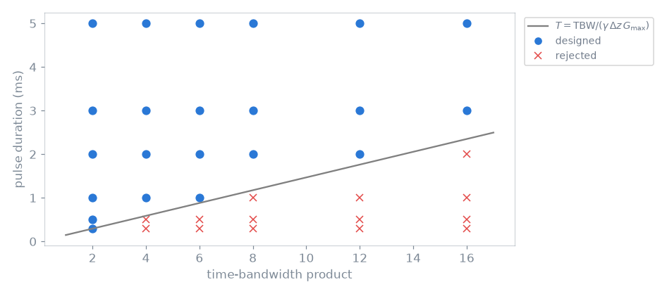
22 of 36 designs realizable, 14 rejected

The designs the module accepted are exactly those above the line. The bound is on the amplitude alone: changing the slew limit over the range a gradient system covers moves none of the points across it, because a lower slew rate lengthens the ramps on either side of the selection plateau, and hence the duration of the module, without changing the plateau amplitude.

The same plane read along its other axis gives the complementary statement: a sharper profile at a fixed slice thickness is available at any duration the gradient amplitude supports, and choosing between a long pulse and a strong gradient determines the echo time and the peak \(B_1\) rather than the profile.