Readout modules

The previous lesson replaced the hand-built excitation with a module. This lesson replaces the hand-built readout of the first sections with the readout module, and uses two prescriptions that the earlier lessons solved by hand — a partial echo and a multi-echo train — to check that the module reaches the same results and reports them.

A readout module takes the system limits, the excitation pulse of the repetition and a prescription, and solves the gradients, the acquisition window and the timing from them. The order in which lines are acquired is not part of the module; it belongs to the loop, which is the subject of A sequence application. The module concept, and the reason the design is divided in this way, are described in Sequence modules.

Learning objectives

After this lesson, you should be able to:

• design a readout with the readout module and read its events, timing, sampling and achieved receiver bandwidth;

• play the blocks of the module into a sequence for one repetition;

• relate the partial-echo fraction to the shortest echo time, as measured by hand in Gradient echo;

• explain why the achieved receiver bandwidth depends on the number of samples;

• compare monopolar and bipolar multi-echo trains.

What a module holds

The excitation module designs the pulse, its selection gradient and the rephaser; the readout module takes those and the prescription. With the echo time unset, the module uses the shortest echo time the prescription allows. The achieved receiver bandwidth is constrained by the rasters and can differ from the requested one; the module reports the achieved value.

import pypulseqpp as pp
import pypulseqpp.sequences as design

system = pp.Opts(
    max_grad=40.0,
    grad_unit="mT/m",
    max_slew=150.0,
    slew_unit="T/m/s",
    rf_dead_time=100e-6,
    rf_ringdown_time=20e-6,
    adc_dead_time=10e-6,
)

FOV = 220e-3
MATRIX = 128
THICKNESS = 5e-3
FLIP_ANGLE_DEG = 12.0

excitation = design.SpatialSelectiveExcitation(
    system, FLIP_ANGLE_DEG, THICKNESS, duration_s=3e-3, time_bw_product=4.0
)
readout = design.LineReadout2D(
    system,
    excitation.rf,
    excitation.gz,
    excitation.gz_reph,
    fov=(FOV, FOV),
    matrix=(MATRIX, MATRIX),
    te=None,
    readout_bandwidth_hz=250e3,
    spoiling_cycles=4.0,
)

print(
    f"echo time {1e3 * readout.echo_time:.3f} ms, "
    f"module {1e3 * readout.duration:.3f} ms\n"
    f"{readout.n_samples} samples at {readout.bandwidth_hz / 1e3:.1f} kHz, "
    f"echo on sample {readout.center_sample}, "
    f"line spacing {readout.delta_kx:.2f} 1/m"
)

/home/runner/work/pypulseqpp/pypulseqpp/docs/build/site/pypulseqpp/_events.py:273: UserWarning: Specified RF delay 0.00 us is less than the dead time 100 us. Delay was increased to the dead time.
  made = factory(*args, **kwargs)
echo time 2.800 ms, module 6.480 ms
128 samples at 100.0 kHz, echo on sample 64, line spacing 4.55 1/m

One repetition

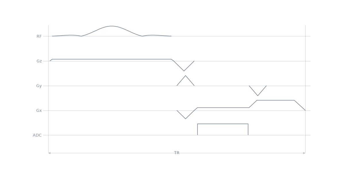
blocks is the module’s playout in order, as tuples of events. A loop adds them to a sequence, scaling the phase-encode template to the line it is acquiring; here the largest step is played, and the pulse’s block is added first because the module is the readout half of the repetition.

seq = pp.Sequence(system=system)
seq.add_block(excitation.rf, excitation.gz)
for block in readout.blocks:
    seq.add_block(*block)

ok, errors = seq.check_timing()
print(f"timing {ok}, {seq.num_blocks} blocks, {1e3 * seq.duration()[0]:.3f} ms")

readout.paper_plot()

timing True, 5 blocks, 9.640 ms

Shortest echo time against partial echo

partial_echo is the fraction of the full echo acquired, and truncates the samples before it. The shortest echo time follows, as it did when the same readout was built by hand: the samples that are no longer taken are the ones that stood between the excitation and the echo.

FRACTIONS = (1.0, 0.875, 0.75, 0.625, 0.5625)


def solved(partial_echo=1.0, bandwidth_hz=250e3, **prescription):
    """One readout module, solved for the shortest echo time."""
    return design.LineReadout2D(
        system,
        excitation.rf,
        excitation.gz,
        excitation.gz_reph,
        fov=(FOV, FOV),
        matrix=(MATRIX, MATRIX),
        te=None,
        partial_echo=partial_echo,
        readout_bandwidth_hz=bandwidth_hz,
        spoiling_cycles=4.0,
        **prescription,
    )


partial = [
    {
        "fraction": fraction,
        "module": solved(partial_echo=fraction),
    }
    for fraction in FRACTIONS
]

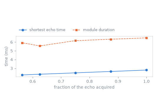
partial echo   samples   echo on      achieved          TE      module
      1.0000       128        64      100.0 kHz    2.800 ms    6.480 ms
      0.8750       112        48      100.0 kHz    2.640 ms    6.320 ms
      0.7500        96        32      100.0 kHz    2.480 ms    6.160 ms
      0.6250        80        16      250.0 kHz    2.324 ms    5.560 ms
      0.5625        72         8      100.0 kHz    2.240 ms    5.920 ms

The sample the echo lands on moves with the fraction, and the echo time falls with it.

The achieved bandwidth is not the requested one at every fraction, and not the same one at every fraction either. A dwell time lies on the ADC raster and an acquisition window on the gradient raster, and whether a given dwell satisfies both depends on how many samples are taken: at 80 samples the requested 250 kHz lands on both rasters and is used, and at the neighbouring counts the fastest rate that does is 100 kHz. That is why the module duration does not fall monotonically while the echo time does, and why the module reports the achieved rate rather than the requested one.

Monopolar against bipolar trains

n_echoes sets the train length, and flyback selects how it is played: a monopolar train rewinds between the echoes so that every one is read in the same direction, and a bipolar train alternates the readout sign, as the hand-built train of Multi-echo readouts did. The bipolar train is shorter by the duration of the rewinders, and its even echoes are read backwards.

ECHOES = 4

trains = {
    "monopolar": solved(n_echoes=ECHOES, flyback=True),
    "bipolar": solved(n_echoes=ECHOES, flyback=False),
}

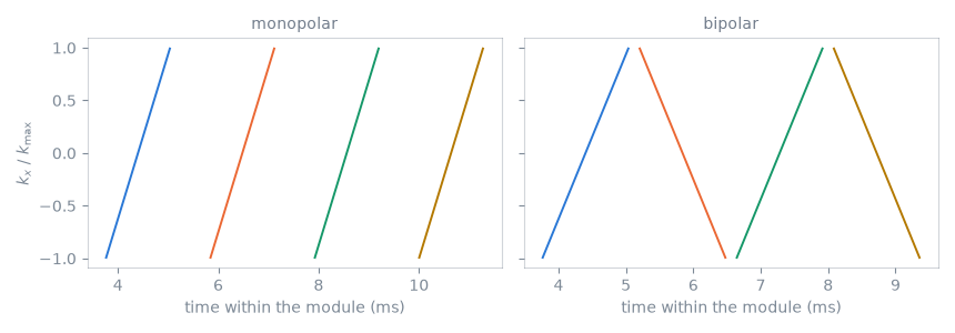
    train    echo spacing    first echo       module
monopolar        2.080 ms      2.800 ms    12.840 ms
  bipolar        1.440 ms      2.800 ms    10.920 ms

Every echo of the monopolar train is traversed in the same direction and the gaps between them are the rewinders; the bipolar train has no gaps and every second echo runs backwards. The choice between them follows from the relationship measured in the earlier lesson: the bipolar train is shorter, and any delay between the gradient and the acquisition enters it as a difference between the odd and the even echoes rather than as a shift common to all of them.