Safety-check computations

What each function in pypulseqpp.safety evaluates, in which frame and units, and over which interval. The concepts are in Safety checks.

Frames and units

A block’s ROTATIONS extension turns its gradients from the channel axes they are stored on to the logical axes. A prescription rotation, composed after each block’s own, turns the logical axes to the physical axes. Every gradient check reads the waveforms after the blocks’ rotations. check_pns(), check_mech_resonance() and check_spl() take the prescription as rotation, a 3x3 orthonormal matrix. The amplitude, slew-rate and continuity checks read the rotations the sequence holds; a prescription is applied to them with TransformFOV before checking.

Check	Report unit	Interval
amplitude, slew rate, continuity	Hz/m, Hz/m/s (system.gamma converts)	every sample
PNS	fraction of threshold	whole sequence, from rest
mechanical resonance	mT/m	sliding windows
sound pressure	dB, dB(A)	the loudest repetition, periodic
SAR	W/kg	each repetition

Every check returns (is_ok, report); the report is returned whether or not the check passes.

Gradient amplitude and slew rate

check_max_grad() evaluates

\[ \max_{t}\;\max_{a \in \{x,y,z\}} |G_a(t)| \;\le\; \mathtt{max\_grad}, \]

and reports each axis peak with its 1-based block and the largest simultaneous vector magnitude \(\max_t |\mathbf{G}(t)|\). Only the per-axis quantity is compared, because max_grad in a Pulseq system description is a per-axis limit. check_max_slew() does the same for \(\mathrm{d}G_a/\mathrm{d}t\) within each block: for a trapezoid, the amplitude over the ramp time; for an arbitrary gradient, the difference between neighbouring samples over their spacing on the gradient raster. A nonpositive limit disables its comparison.

A readout traversing \(\Delta k = N/\mathrm{FOV}\) in a window \(T\) needs \(G = \Delta k / T\) in Hz/m. For an area \(A\) at slew rate \(S\), the shortest lobe is a triangle of peak \(\sqrt{AS}\) and duration \(2\sqrt{A/S}\); above max_grad it acquires a flat top.

apply_system_derates() returns a copy of the system limits with max_grad and max_slew scaled from base values the copy retains, so derating does not compound; cap_system() lowers them to stated ceilings.

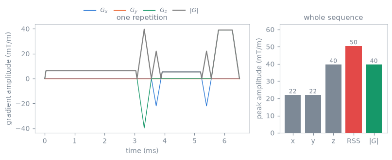
A radial gradient echo. The root-sum-square of the three axis peaks is larger than the largest simultaneous vector magnitude, because the axes peak at different times.

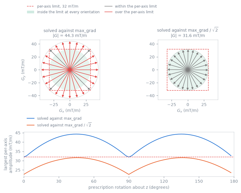
The in-plane gradient vector of a Cartesian gradient echo at the instant its magnitude is largest, at prescription rotations 15 degrees apart. Left, solved against max_grad, with both axes at the limit: only diagonal orientations keep both components inside. Right, solved against max_grad divided by \(\sqrt2\). Below, the largest per-axis amplitude against the prescription angle.

Gradient continuity

check_grad_continuity() compares, on each axis after the blocks’ rotations, the last amplitude of a block with the first of the next:

\[ |\Delta G| \leq \mathtt{max\_slew} \cdot \mathtt{grad\_raster\_time}. \]

It reports the 1-based block, axis, both amplitudes and the implied slew rate. The final amplitude on every axis must be zero, or ends_at_zero and the verdict are false. check_timing() reports the same as GRADIENT_DISCONTINUITY and GRADIENT_NOT_RAMPED_DOWN.

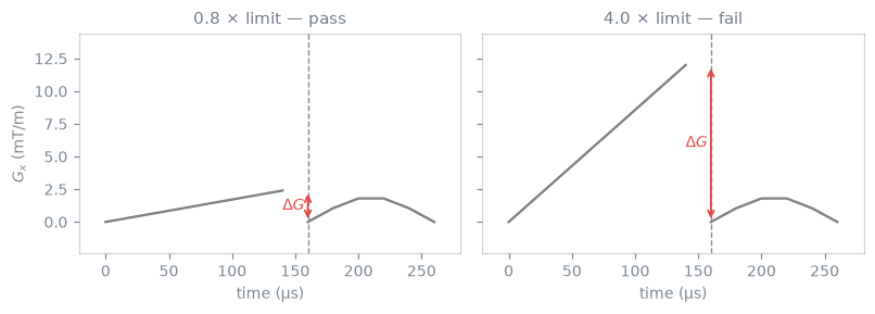
A boundary step below the one-raster limit passes; a larger step is reported.

Peripheral nerve stimulation

For a rectangular stimulus of duration \(\tau\), the chronaxie threshold is \(S(\tau) = S_{\mathrm{rh}}(1 + c/\tau)\), with rheobase \(S_{\mathrm{rh}}\) and chronaxie \(c\).[1]

Model	Coefficients	Source
ChronaxieModel	one chronaxie; rheobase and alpha for all axes or per physical axis	stated, or measured on the coil
SAFE	three exponential terms, amplitude scale and stimulation limit per axis	Siemens .asc, read by read_safe_model()

Each physical axis’s slew waveform drives its response \(R_a(t)\), and \(R(t) = \sqrt{R_x^2 + R_y^2 + R_z^2}\). The check fails where \(R\) exceeds the threshold fraction. The response depends on the preceding slew history, so the sequence is evaluated in one pass from rest. With equal coefficients on every axis a rotation leaves \(R\) unchanged; per-axis coefficients make it depend on the prescription.

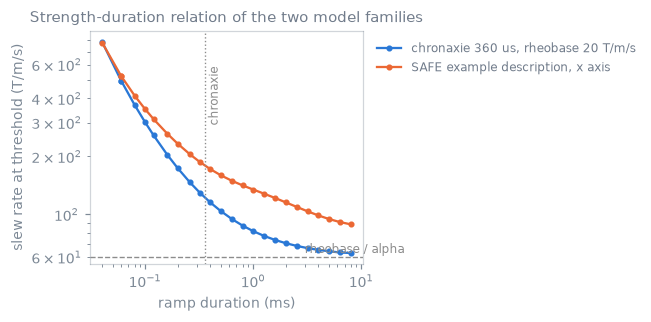
Slew rate at unity response for a demonstration chronaxie model and the PyPulseq SAFE example hardware description.

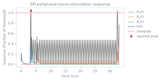
Axis responses, combined response, threshold and reported peak for one EPI acquisition under a synthetic chronaxie model.

Mechanical resonance

Each physical axis is sampled at the centres of the sequence’s gradient raster. A window of window_width (40 ms by default) starts every stride (half a window by default); the last is zero-filled to the end. Each window is mean-subtracted, multiplied by a Hann taper \(w\), zero-padded to frequency_oversampling (3) times its length and transformed, with

\[ A_k = \frac{2\,|X_k|}{\sum_n w_n}, \]

so a sustained sinusoid of amplitude \(A\) at a bin frequency reads \(A\) in mT/m. The check evaluates only the bins a band reads, as direct sums; mech_resonance_spectrum() returns every bin of one window from a real FFT of the same samples.

A ForbiddenBand is an axis (None for all three), an inclusive range in Hz and a tolerance in mT/m. The threshold is the tolerance where positive and min_threshold (10 mT/m) otherwise. A band is violated by each window whose largest amplitude on a bin inside it exceeds the threshold on any axis it guards; a band narrower than a bin is read at the bin nearest its centre. The report keeps each band’s worst window. read_forbidden_bands() reads the acoustic resonances of a Siemens .asc file as centre ± bandwidth/2 on all axes, tolerance 0.

A train alternating at echo spacing \(\Delta t\) has its fundamental at \(1/(2\,\Delta t)\), with an amplitude between \(8/\pi^2\) (triangular) and \(4/\pi\) (square) of the plateau, and odd harmonics. A tolerance stated as a plateau amplitude is compared unscaled with this spectral amplitude.[2] The criterion applies to the commanded waveform; it models neither the coil’s transfer function nor its acoustic output.

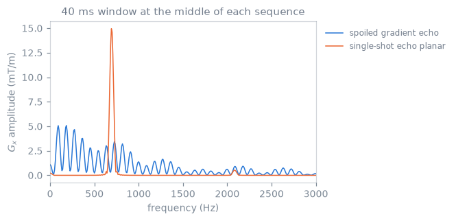
The readout-axis spectrum of a 40 ms window at the middle of two 64 x 64 sequences: a spoiled gradient echo and a single-shot echo-planar train.

Sound pressure

check_spl() takes the repetition of repetition(), counted from block 1, over which the squared gradient summed over the axes integrates to the most, the earliest on a tie. It filters that repetition by the acoustic transfer function of each physical axis as a periodic waveform and reports the peak in dB, the A-weighted RMS in dB(A) and the unweighted RMS in dB, against 140 dB and 99 dB(A) by default (IEC 60601-2-33). A sequence without gradients reads -inf. read_acoustic_response() reads the transfer function from HDF5, per mT/m on its positive bins.

SAR

Local SAR at a position, for channel phasors \(\mathbf{v}\), is \(\mathbf{v}^{\mathsf H} Q \mathbf{v}\). VOPs \(\{Q_k\}\) bound the largest value over the body model by \(\max_k \mathbf{v}^{\mathsf H} Q_k \mathbf{v}\).[3] VopModel holds the \((N, N_c, N_c)\) stack in W/kg per unit drive squared, optional global matrices (one, or one per body model) and metadata whose safety_factor \(M \geq 1\) multiplies local SAR. read_vops() reads .mat and .npz, point-first and channel-first, including mariepy’s population files.

Channel \(c\) is driven with \(v_c(t) = d_c\,s_c\,b_c(t)\): drive_per_hz, the block’s RF shim (or default_shim for a single-channel pulse, played on every channel) and the RF waveform in Hz resampled every microsecond, as calc_rf_power() does. In a window \(W\) of duration \(T_W\),

\[ \mathrm{SAR}_{\mathrm{local}}(W) = \frac{M}{T_W} \max_k \int_W \mathbf{v}^{\mathsf H} Q_k\, \mathbf{v}\,\mathrm{d}t, \]

and global SAR is the same integral with the global matrix, the largest over the body models. The windows are consecutive repetitions of tr_size blocks (repetition(), or a TRSize definition the blocks repeat with); blocks before the first repetition form a window of their own, and a sequence that does not repeat is one window. Limits default to 10 W/kg local and 3.2 W/kg global (IEC 60601-2-33 normal mode, head). The report gives each window’s blocks, duration, local SAR, VOP index, global SAR and body model. No regulatory averaging interval is applied.

Reference-pulse ratios

With reference, the reference is played under the same model, drive and default shim. With \(\mathrm{SAR}^{\mathrm{ref}}_{G_b}\) its global SAR in body model \(b\), in its window of largest global SAR of duration \(T^{\mathrm{ref}}\),

\[ r_{\mathrm{local}} = \max_W \frac{\mathrm{SAR}_{\mathrm{local}}(W)}{\min_b \mathrm{SAR}^{\mathrm{ref}}_{G_b}}, \qquad r_{\mathrm{global}} = \max_{W,b} \frac{\mathrm{SAR}_{G_b}(W)}{\mathrm{SAR}^{\mathrm{ref}}_{G_b}}, \]

reported as local_to_head and global_sar_ratio; with each window’s term times \(T_W/T^{\mathrm{ref}}\), as local_to_head_energy and global_energy_ratio; per window in windows.local_to_head and windows.global_ratio. The smallest reference SAR over the body models sets the largest drive scale, so it sets the local term. The global term is taken body by body, because a subject’s global SAR is that of one body.

If the scanner holds the reference at the global limit \(L_G\) at its shortest repetition time, a window’s local SAR is at most \(r_{\mathrm{local}} L_G\), and the sequence meets both limits when each repetition lasts at least

\[ T^{\mathrm{ref}} \max\!\left(r^{E}_{\mathrm{global}},\; r^{E}_{\mathrm{local}}\,\frac{L_G}{L_L}\right), \]

with \(L_L\) the local limit. This rests on the scanner’s prediction for the reference not falling below its true global SAR, and on the VOPs and safety factor bounding local SAR. The scale of drive_per_hz and of the matrices cancels; relative channel gains and the safety factor do not. A report of an earlier call can stand for the reference.

example_vops() is a synthetic eight-channel loop array around a uniform cylinder, with no tissue, coupling or conservative field.

References

[1]

Irnich W, Schmitt F. Magnetostimulation in MRI. Magnetic Resonance in Medicine. 1995;33(5):619–623. doi:10.1002/mrm.1910330418.

[2]

Hedeen RA, Edelstein WA. Characterization and prediction of gradient acoustic noise in MR imagers. Magnetic Resonance in Medicine. 1997;37(1):7–10. doi:10.1002/mrm.1910370103.

[3]

Eichfelder G, Gebhardt M. Local specific absorption rate control for parallel transmission by virtual observation points. Magnetic Resonance in Medicine. 2011;66(5):1468–1476. doi:10.1002/mrm.22927.