1. Your first gradient echo

This course takes you from a 2D Cartesian gradient echo to a 3D radial MPRAGE, one step per lesson. This lesson starts with the gradient echo.

It covers the Pulseq basics: you describe your scanner, design the events of one repetition (the excitation, the readout, the phase encoding), play them in blocks, one k-space line per repetition, and write the file the scanner plays. If you have written PyPulseq before, every line will look familiar: pypulseqpp keeps PyPulseq’s names, arguments and units.

Learning objectives

• Describe your scanner with a system object, and know which raster each event is aligned to.

• Design every event once, before the loop, from the field of view and the matrix.

• Play one repetition per k-space line in blocks, and check the timing.

• Read the sequence diagram and the k-space trajectory, and write the .seq file.

Next: 2. Echo and repetition time, where you place the echo at the echo time you ask for.

Repetition structure

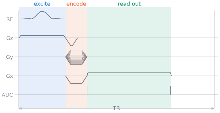
Each repetition (each TR) of the sequence consists of three steps:

1. Excite one slice. A sinc pulse is played together with a gradient along z, so only the spins in the slice are on resonance.

2. Encode. A phase-encoding gradient along y moves k-space to the line this repetition acquires, and a prewinder along x moves it to the start of that line.

3. Read out. A gradient along x sweeps the line while the ADC samples it. The echo forms in the middle of the readout, where the readout gradient has undone the prewinder.

The scan repeats this once per line, changing only the phase-encoding amplitude. By the end of the lesson your sequence draws this diagram:

System limits

Before you design anything, you tell pypulseqpp what your scanner can do. This is the system object, a Opts: the gradient amplitude and slew-rate limits, and the dead times the RF and receive chains need around an event. Every factory below designs its event against it, so the same code gives you a different, but always playable, event on a different scanner. Anything you leave out keeps its default.

import numpy as np

import pypulseqpp as pp

system = pp.Opts(
    max_grad=32.0,
    grad_unit="mT/m",
    max_slew=130.0,
    slew_unit="T/m/s",
    rf_dead_time=100e-6,
    rf_ringdown_time=20e-6,
    adc_dead_time=10e-6,
)

The scanner does not play arbitrary times: each kind of event starts and changes on its own clock, its raster. Gradient waveforms are defined on the gradient raster, RF samples on the RF raster, ADC dwell times on the ADC raster, and every block lasts a whole number of block-duration rasters. They are part of system too:

print(f"gradient raster {1e6 * system.grad_raster_time:g} us")
print(f"RF raster       {1e6 * system.rf_raster_time:g} us")
print(f"ADC raster      {1e6 * system.adc_raster_time:g} us")
print(f"block raster    {1e6 * system.block_duration_raster:g} us")

gradient raster 20 us
RF raster       2 us
ADC raster      2 us
block raster    20 us

The factories place every event they design on its raster. Times you choose yourself, such as a delay, a dwell time or an echo time, have to be placed on the raster explicitly.

Protocol

A field of view of 220 mm, a 128 by 128 matrix, a 5 mm slice, a 12 degree flip angle and a TR of 20 ms. The field of view and the matrix fix k-space: lines are \(1/\mathrm{FOV}\) apart, and each line spans \(N/\mathrm{FOV}\).

FOV = 220e-3
MATRIX = 128
THICKNESS = 5e-3
FLIP_ANGLE_DEG = 12.0
TR = 20e-3

delta_k = 1 / FOV

Excitation

make_sinc_pulse() designs a slice-selective sinc pulse. You give it the flip angle, the duration, the slice thickness and the time-bandwidth product, and with return_gz=True it also returns the slice-selection gradient and the rephaser, a short negative gradient that undoes the phase the slice accumulates under the second half of the selection gradient. Without the rephaser the signal across the slice would cancel out.

The delay starts the pulse after the RF dead time, and use="excitation" records the role of the pulse for the interpreter and the k-space analysis.

rf, gz, gz_reph = pp.make_sinc_pulse(
    flip_angle=np.deg2rad(FLIP_ANGLE_DEG),
    duration=2e-3,
    slice_thickness=THICKNESS,
    apodization=0.5,
    time_bw_product=4.0,
    delay=system.rf_dead_time,
    system=system,
    use="excitation",
    return_gz=True,
)

Readout

The readout gradient has to sweep one whole line, \(N\,\Delta k\), while the ADC samples it at constant amplitude, so you ask for the area of its flat top and for a flat time that holds the samples. The time between two samples is the dwell time, and its inverse is the receiver bandwidth.

You want a dwell of about 26 µs, and the dwell has to be on the ADC raster. A dwell off the raster is rejected by the timing check. With 25.9 µs, one readout gives:

dwell = 25.9e-6
gx = pp.make_trapezoid(
    "x", flat_area=MATRIX * delta_k, flat_time=MATRIX * dwell, system=system
)
adc = pp.make_adc(MATRIX, dwell=dwell, delay=gx.rise_time, system=system)

seq = pp.Sequence(system)
seq.add_block(gx, adc)
ok, errors = seq.check_timing()
print(f"timing ok: {ok}")
for error in errors:
    print(f"  block {error.block}, {error.event}.{error.field}: {error.error_type}")

timing ok: False
  block 1, gx.flat_time: RASTER
  block 1, adc.dwell: RASTER

check_timing() walks every block and reports each event that is off its raster or too close to a dead time. Here the flat time of the gradient and the dwell time of the ADC are both off. Neither is wrong by much, but the scanner cannot play them.

calc_adc_timing() resolves this: it moves the requested dwell onto the ADC raster, and returns a readout duration that ends on the gradient raster. The ADC starts after the gradient’s ramp (delay=gx.rise_time), so every sample is taken on the flat top.

dwell, readout_time = pp.calc_adc_timing(
    MATRIX,
    26e-6,
    grad_raster_time=system.grad_raster_time,
    adc_raster_time=system.adc_raster_time,
)
gx = pp.make_trapezoid(
    "x", flat_area=MATRIX * delta_k, flat_time=readout_time, system=system
)
adc = pp.make_adc(MATRIX, dwell=dwell, delay=gx.rise_time, system=system)

print(
    f"dwell {1e6 * dwell:.0f} us, receiver bandwidth {1e-3 / dwell:.1f} kHz, "
    f"{1 / (dwell * MATRIX):.0f} Hz per pixel"
)

dwell 30 us, receiver bandwidth 33.3 kHz, 260 Hz per pixel

You asked for 26 µs and got the closest dwell at or above it for which both conditions hold. A longer dwell means a lower receiver bandwidth, a longer readout and a higher signal-to-noise ratio.

The prewinder moves k-space from the centre to the start of the line, so the readout crosses the centre halfway through: it is a gradient along x with minus half the readout’s area. You also ask for its duration, 1 ms, so it fits in the same block as the phase encoding.

gx_pre = pp.make_trapezoid("x", area=-gx.area / 2, duration=1e-3, system=system)

Phase encoding

Each repetition acquires a different line, \(k_y = m\,\Delta k\) with \(m\) from \(-N/2\) to \(N/2 - 1\). You design one phase-encoding gradient, the largest, and in the loop you only scale it with scale_grad().

gy_pre = pp.make_trapezoid("y", area=MATRIX / 2 * delta_k, duration=1e-3, system=system)
phase_steps = np.arange(-MATRIX // 2, MATRIX // 2) / (MATRIX / 2)

This is the main rule of writing a Pulseq sequence: design every event once, before the loop. A factory solves for the shortest waveform that does what you ask, and solving it again in every repetition costs time and produces nothing new. Inside the loop, only the amplitudes and phases of existing events change. The scan then reuses the same few waveforms, and the file stores each of them once.

Scan loop

One repetition is four blocks. A block holds at most one event per channel (RF, ADC and each gradient axis), all of them start together, and the block lasts as long as its longest event. Blocks play one after the other.

1. the pulse and the slice-selection gradient;

2. the prewinder, the phase encoding and the rephaser, which do not interfere and so play together;

3. the readout gradient and the ADC;

4. a delay that fills the rest of the TR.

The delay is what you choose yourself, so you put it on the block-duration raster with round_to_raster().

played = (
    pp.calc_duration(rf, gz)
    + pp.calc_duration(gx_pre, gy_pre, gz_reph)
    + pp.calc_duration(gx, adc)
)
tr_delay = pp.round_to_raster(TR - played, system.block_duration_raster)

seq = pp.Sequence(system)
for step in phase_steps:
    seq.add_block(rf, gz)
    seq.add_block(gx_pre, pp.scale_grad(gy_pre, step), gz_reph)
    seq.add_block(gx, adc)
    seq.add_block(pp.make_delay(tr_delay))

ok, errors = seq.check_timing()
print(f"timing ok: {ok}, {seq.num_blocks} blocks, scan time {seq.duration()[0]:.2f} s")

timing ok: True, 512 blocks, scan time 2.56 s

Sequence diagram

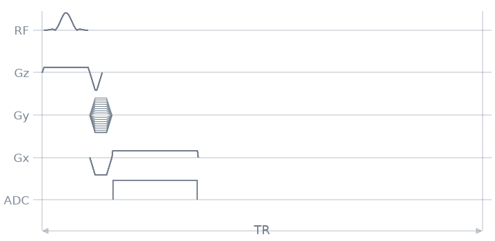
paper_plot() draws one repetition, one row per channel. The solid trace is the repetition you pick (here the first); the shaded traces are all the others, so you can see what changes from one TR to the next: only the phase-encoding amplitude.

seq.paper_plot(tr=1)

k-space trajectory

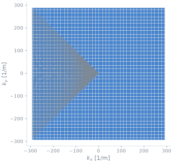
pypulseqpp.plot.plot_kspace() integrates the gradients from each excitation and marks where the ADC samples. Each repetition jumps to its line during the prewinder and sweeps it left to right during the readout: 128 lines on a Cartesian grid, \(\Delta k\) apart.

pp.plot.plot_kspace(seq, plane="xy")

Pulseq file

Last, you write the file the scanner plays. The definitions you set go in its header, next to the blocks; a reconstruction reads them to know what was acquired. Lesson 4 covers them in detail.

from pathlib import Path
from tempfile import mkdtemp

seq.set_definition("Name", "gre")
seq.set_definition("FOV", [FOV, FOV, THICKNESS])
path = Path(mkdtemp()) / "gre.seq"
seq.write(str(path))
print("\n".join(path.read_text().splitlines()[:8]))

# Pulseq sequence file
# Created by PyPulseq

[VERSION]
major 1
minor 5
revision 1

Any Pulseq interpreter plays this file. What it holds (blocks, events and shared libraries of shapes), and the rasters its times lie on, are explained in Pulseq file format.

Specification

What this lesson built, stated the way you would ask an agent for it:

Write a pypulseqpp 2D Cartesian gradient echo for a scanner with
32 mT/m and 130 T/m/s, 100 us RF dead time, 20 us RF ringdown and
10 us ADC dead time. Protocol: 220 mm FOV, 128x128 matrix, one 5 mm
slice, 12 degree sinc excitation (2 ms, time-bandwidth product 4),
about 26 us dwell, TR 20 ms. Design every event before the loop,
scale the phase encoding in the loop, put the TR delay on the block
raster, check the timing, and write gre.seq with the Name and FOV
definitions.