RF and gradient design internals

The rules, units and algorithms behind the designers. The concepts are in RF and gradient design.

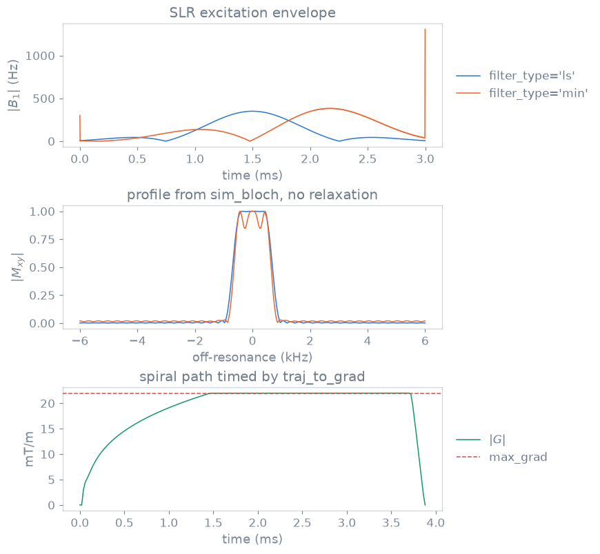
Linear-phase and minimum-phase SLR excitations of time-bandwidth product 4 and duration 3 ms, their profiles from sim_bloch, and a spiral timed by traj_to_grad at 22 mT/m and 150 T/m/s.

Units and rasters

RF amplitudes are in Hz, frequency offsets in Hz, phase offsets in rad, flip angles in rad and durations in s. B1 amplitudes that are inputs of the B1 designers are in T, and the returned events are in Hz. Gradient amplitudes are in Hz/m, slew rates in Hz/m/s and k-space in 1/m, on the channel axes. RF samples lie on the RF raster (dwell, the system’s rf_raster_time when zero) and gradient waveforms on the gradient raster. make_wave_gradients takes its amplitude in T/m. The solver behind traj_to_grad works internally in Hz per pixel and its output is converted before it is returned.

Shinnar-Le Roux designs

make_slr_pulse() follows SigPy’s sigpy.mri.rf.slr and sigpy.util.leja, and through SigPy Pauly’s rf_tools; the SLR design is in pypulseqpp._slr in NumPy and SciPy, and the exhaustive root-flip search in pypulseqpp._ext.slr (BSD 3-Clause, LICENSES/SigPy-BSD-3-Clause.txt).

Parameter	Values
pulse_type	st small-tip, ex excitation, se spin echo, inv inversion, sat saturation
filter_type	ls least squares, pm Parks-McClellan, min minimum phase, max maximum phase (the time reverse of min), ms windowed sinc

The passband and stopband ripples are converted per pulse type before the filter is designed: ex uses \(\delta_1 \to \sqrt{\delta_1/2}\) and \(\delta_2 \to \delta_2/\sqrt{2}\), se \(\delta_1/4\) and \(\sqrt{\delta_2}\), inv \(\delta_1/8\) and \(\sqrt{\delta_2/2}\), and sat \(\delta_1/2\) and \(\sqrt{\delta_2}\). A duration that spans fewer than four RF samples is refused.

Effective centre. center_pos, in \([0, 1]\) of the duration, is the centre the event records and the point the slice-select rephaser refocuses from. It defaults to the magnitude peak of the designed waveform, as calc_rf_center() finds it. A minimum-phase pulse is used at center_pos=1.0, its own end. The rephaser area follows from the centre, and so does the echo time a readout module measures from it.

Root flipping. With root_flip=True the roots of the SLR beta polynomial are flipped to minimise the peak B1 for the same profile magnitude (Sharma, Lustig and Grissom, 2016); the profile phase is then no longer linear.

• It needs a pulse_type with a nominal flip, so a small-tip pulse is refused.

• It is refused together with cancel_alpha_phase.

• It visits every subset of the passband’s roots, \(2^n\) patterns, and refuses a passband with more than 30 candidates.

• The compiled search selects the pattern an exhaustive NumPy search selects, and does not depend on the number of threads sharing it.

• The roots are Leja-ordered, a permutation that starts from the largest.

• The pulse plays at its designed amplitude scaled by flip_angle over the nominal flip, not by area. A design of more than 256 samples is searched at 256 samples and resampled, so it keeps the coarse design’s profile.

Related designs.

Function	Rule
make_recursive_slr_pulses()	One pulse per segment with flips that grow to 90 degrees at the last, so each excites the same transverse magnetisation of non-recovering magnetisation; with use_mz each is designed against the longitudinal profile the earlier ones left (SigPy’s dz_recursive_rf). The SLR core spans about duration / 1.75, a Blackman taper fills the rest. The pulses play at their designed amplitude.
make_sms_pulse()	The envelope is multiplied by \(\sum_b w_b e^{2\pi i f_b t}\) with \(t\) from the start of the shape, so band phases are referenced to the start, not the centre. Offsets always include 0 Hz; for an even band count the unpaired band is on the positive side. Sideband power is power: weights take its square root. Phase schedules: quadratic (Grissom), wong (3 to 16 bands), malik (4 to 12 bands, which makes the modulation of symmetric bands real).
make_spsp_pulse()	An SLR envelope on an alternating gradient that ends balanced; a slab too thin for the slew lengthens its ramps only as far as the slew needs, and one the hardware cannot do is refused.
make_2d_selective_pulse()	Small-tip design on a centre-out spiral, each interleaf followed by an RF-off retrace to the origin, arc-length weighting without a radial density factor, so no rephaser is needed. fov is square and the profile repeats with period fov.

Adiabatic pulses

make_adiabatic_pulse() builds hypsec (Baum, Tycko and Pines 1985) and wurst (Kupce and Freeman 1995) through PyPulseq’s factory, and bir4 (Staewen et al. 1990) and goia_wurst (Andronesi et al. 2010) itself. For every sweep the amplitude meets adiabaticity where the frequency sweep crosses zero:

\[ (\gamma B_1)^2 = \mathtt{adiabaticity}\,\left|\frac{d\omega}{dt}\right| \quad (\text{rad/s}). \]

• bir4 rotates by flip_angle through the phase jumps between the quarters of two BIR-1 halves, with kappa shaping \(\tan(\kappa s)/\tan\kappa\) over each quarter; it selects no slice and refuses a gradient.

• goia_wurst modulates its gradient with the sweep, so every position in the slice sees the same adiabaticity: \(G/G_{\max} = (1 - m) + m\,|\cos(\pi t/T)|^{p}\) with \(G_{\max} = \mathtt{bandwidth}/\mathtt{slice\_thickness}\), \(m\) = gradient_modulation and \(p\) = gradient_order. It requires return_gz and a positive slice_thickness, and starts no earlier than its gradient’s ramp ends.

• BIR-4 and GOIA-WURST are referenced to zero phase at the crossing and use a multiple of four samples, zero-padded to duration; fewer than eight samples is refused. The WURST truncation \(1 - |\cos(\pi t/T)|^{n}\) has \(n\) = 40 for wurst and 16 for goia_wurst.

• make_half_passages() returns down, the first half of a sweep, and up, down time-reversed and conjugated, so the phase accrued on the way down unwinds on the way up. The default adiabaticity is 8, twice an inversion’s, because a half passage has half a sweep to converge in.

B1-encoding pulses

make_bloch_siegert_pulse() plays a constant amplitude with its frequency swept from far off resonance towards it and back, symmetric about the centre. Longitudinal magnetisation stays on \(z\) and transverse magnetisation gains a phase proportional to \(B_1^2\) (Khalighi, Rutt and Kerr, Magn Reson Med 70:829, 2013); playing the sweep on either side of resonance and differencing the phases maps B1. duration is rounded to an even number of RF samples. The sweep \(\gamma B_1 t/k\) must stay below one over half the pulse, or the design is refused. The preparation module plays it alone in its block, unspoiled. make_b1_selective_pulse(), make_b1_gslider_pulse() and make_b1_hadamard_pulse() take the amplitude in T and a relative passband.

Parallel transmit

A dynamic pTx pulse is one arbitrary RF event holding every transmit channel’s waveform one after another over a shared time base, so its time shape restarts once per channel (Roos et al., Magn Reson Med 2025, doi:10.1002/mrm.30601).

• The channel count is the number of samples at the first sample time, as the reference interpreter reads it, and is accepted only when the times are that many identical copies; anything else is one channel. The rule is rf_channels in src/cpp/pulseq/channels.hpp.

• make_ptx_pulse() writes the layout from (channels, samples) complex waveforms in Hz, played as given: nothing is scaled to a flip angle, since with several channels the flip depends on each channel’s B1 map. split_ptx_pulse() reads it back.

• shape_dur is one channel’s duration, so an interpreter unaware of the layout reads the right length, and the core’s timing check judges one channel’s time base. A waveform that is not two-dimensional, holds no samples or has a time base that does not repeat is refused.

• Flip-angle integrals take each channel on its own time base and sum them, the flip where every channel has unit, in-phase sensitivity. RF power sums \(|b_c|^2\) over the channels at each time.

• The pulse centre defaults to the peak of the root sum square of the channels’ magnitudes. The bandwidth is that of the sum of the channels.

• The layout survives writing and reading, and upstream reads the same channels.

RF shim. make_rf_shim() creates the rf_shim extension event, complex weights one per channel, stored as complex128; a block carries at most one, and blocks shimmed alike share one library row. calc_rf_shim() fits magnitude least squares of \(\sum_c w_c b_{1,c}\) over a mask with free phase, with optional Tikhonov weight on \(\sum|w|^2\), starting from the channel combination that delivers the most field over the mask and stopping at a relative cost change of tolerance or after rounds phase exchanges. The B1+ maps may be in any unit shared by all channels.

Spokes and 2D-selective pTx. The design kernels, in src/cpp/bindings/ptx.cpp, follow SigPy’s sigpy.mri.rf.ptx and shim (BSD 3-Clause): the spatial-domain method of Grissom et al. (Magn Reson Med 56:620, 2006) solved by conjugate gradients with magnitude-least-squares phase updates, and greedy spoke selection (Grissom et al., Magn Reson Med 68:1553, 2012). make_spokes_pulse() plays one small-tip SLR sub-pulse per lobe of an alternating slice gradient, with in-plane blips between lobes; one spoke sits at the k-space centre, candidate positions span 1 / resolution at a pitch of 1 / fov, and the per-channel weight of each spoke is fitted to a uniform flip_angle over the mask. The b1_maps are relative, a map of ones being nominal amplitude; the model is the small-tip approximation.

Bloch simulation

sim_bloch() rotates the magnetisation in each hard-pulse step right-handedly about \((\mathrm{Re}\,b_1, \mathrm{Im}\,b_1, b_z)\) by \(2\pi\,\Delta t\) times that vector’s length. There is no relaxation. Each position’s steps compose as SU(2) elements in src/cpp/bindings/sim.cpp and are converted to one rotation at the end, over a worker per chunk of positions.

Argument	Shape and unit
b1_hz	\((T,)\) shared or \((P, T)\) per position, complex, Hz
bz_hz	\((P, T)\), or \((P, 1)\) held throughout, Hz; its rows define the positions
dt	step, s
initial	\((3,)\) or \((P, 3)\), \(+z\) by default

The result is \((P, 3)\); fields whose shapes disagree on positions or steps are refused. sim_rf() follows MATLAB Pulseq’s simRf as a quaternion composition, with no selection gradient, so frequency maps to position only for a constant selection gradient; it returns \(M_z\), \(M_x + iM_y\) from \(+z\), \(+x\) and \(+y\), the frequency axis and a complex refocusing efficiency whose phase is twice the azimuth of the refocusing axis. A ppm offset on the pulse is read against the default system’s gamma and \(B_0\), with a warning.

Arbitrary gradients from a k-space path

traj_to_grad() takes a path as geometry, time last: shape \((n,)\), \((2, n)\) or \((3, n)\) in 1/m, and returns the gradient in Hz/m and the slew rate in Hz/m/s. By default MRArbGrad (Luo, Huang, Miao, Xu, Hu and Qi, IEEE Trans Biomed Eng 2026) finds the gradient that traces it in least time without leaving the vector amplitude and slew limits anywhere along it:

• the output length differs from the input’s, and resampling the same path does not change the gradient;

• oversampling is the path-resampling factor the solver works at, and start_at_zero and end_at_zero ramp the waveform from and to zero;

• the solver works in three dimensions, so a single axis rides in one of a pair and the requested dimensions are returned;

• with time_optimal=False the samples already lie on the raster and are differentiated, as upstream does, with no limit enforced; the slew is averaged back onto the gradient samples and the output is one gradient sample shorter than the path.

calc_spiral_trajectory() and calc_rosette_trajectory() return geometry only, a polyline with no time parameterisation; make_arbitrary_grad wraps one axis of the result as an event. calc_ramp is a separate minimum-time connection of two k-space points under a fixed raster.

The vendored solver. external/MRArbGrad is a submodule of a fork of RyanShanghaitech’s MRArbGrad, MIT licensed, pinned to one commit. Three of its files are compiled (mag/Mag.cpp, utility/global.cpp, utility/v3.cpp) and the rest is headers pulled in by src/cpp/bindings/arbgrad.cpp, the binding pypulseqpp._ext.arbgrad; its own Python package is not built. The shot ordering and rotation a scan replays a base arm under are Python policy. A constant-pitch spiral needs no separate trajectory, since the variable-density one reduces to \(\rho = k_{\rho\phi}\,\phi\) when its two shape parameters are equal. tests/test_arbgrad_spiral.py reports whether the waveforms moved after the submodule is bumped; see external/NOTICE.md.

The designers compute events and profiles from a model, and the checks of Safety checks read the events as played. A simulated profile does not establish how a pulse behaves on a scanner.