4. Labels and metadata

The scanner plays your sequence and hands the reconstruction a stream of readouts. To put each readout in its place, the reconstruction has to know which k-space line it is, which slice, which average, and what the field of view and the matrix are. None of that can be guessed from the samples: you write it into the sequence, as labels on the blocks and definitions in the file header.

In this lesson your gradient echo acquires several slices, so the reconstruction has two things to tell apart, and you label every readout with its line and its slice.

Learning objectives

• Excite several slices by shifting the frequency of the pulse.

• Label each readout with its line and slice, with make_label() and with the Labels helper.

• Write the definitions a reconstruction reads: the field of view, the matrix, TE and TR.

• Read the labels back from the sequence, the way a reconstruction sees them.

Previous: 3. Spoiling. Next: 5. Radial sampling and gradient surgery, where you replace the phase encoding with a rotating readout.

Events

Your spoiled gradient echo from lesson 3, with a smaller matrix so the figures stay readable:

import numpy as np

import pypulseqpp as pp

system = pp.Opts(
    max_grad=32.0,
    grad_unit="mT/m",
    max_slew=130.0,
    slew_unit="T/m/s",
    rf_dead_time=100e-6,
    rf_ringdown_time=20e-6,
    adc_dead_time=10e-6,
)

FOV = 220e-3
MATRIX = 32
THICKNESS = 5e-3
delta_k = 1 / FOV

rf, gz, gz_reph = pp.make_sinc_pulse(
    flip_angle=np.deg2rad(12.0),
    duration=2e-3,
    slice_thickness=THICKNESS,
    apodization=0.5,
    time_bw_product=4.0,
    delay=system.rf_dead_time,
    system=system,
    use="excitation",
    return_gz=True,
)
dwell, readout_time = pp.calc_adc_timing(
    MATRIX,
    26e-6,
    grad_raster_time=system.grad_raster_time,
    adc_raster_time=system.adc_raster_time,
)
gx = pp.make_trapezoid(
    "x", flat_area=MATRIX * delta_k, flat_time=readout_time, system=system
)
adc = pp.make_adc(MATRIX, dwell=dwell, delay=gx.rise_time, system=system)
gx_pre = pp.make_trapezoid("x", area=-gx.area / 2, duration=1e-3, system=system)
gy_pre = pp.make_trapezoid("y", area=MATRIX / 2 * delta_k, duration=1e-3, system=system)
spoiler = pp.make_crusher(4.0, FOV / MATRIX, channel="z", system=system)[0]
phase_steps = np.arange(-MATRIX // 2, MATRIX // 2) / (MATRIX / 2)

Multi-slice acquisition

During the pulse, the slice-selection gradient makes the resonance frequency a function of z: a spin at position \(z\) resonates \(\gamma G_z z\) away from the centre. So to excite a slice at \(z\) you play the same pulse and gradient with the pulse’s frequency shifted by that amount. gz.amplitude is already in Hz/m, so the offset is gz.amplitude * z.

A frequency offset also winds the phase of the pulse. The phase offset that undoes it, measured at the pulse’s centre, keeps every slice in phase.

You acquire three slices, 10 mm apart. Each line is acquired in all three slices before moving to the next line, so the TR, the time between two excitations of the same slice, holds three slots.

SLICES = np.array([-10e-3, 0.0, 10e-3])
SLOT = 20e-3
TR = len(SLICES) * SLOT

rf_centre = pp.calc_rf_center(rf)[0]
slice_frequencies = gz.amplitude * SLICES
slice_phases = -2 * np.pi * slice_frequencies * rf_centre

Labels

A label is an event that sets a counter. Pulseq defines the counters a reconstruction understands, among them LIN (the phase-encoding line), PAR (the partition, in 3D), SLC (the slice), AVG, REP and ECO, and flags such as REV (a readout played backwards) or NAV (a navigator). A label keeps its value until another label event changes it, so you add one only where the value changes, in the block where it does.

make_label() makes one, exactly as in PyPulseq. You put it in the excitation block of every slot, next to the pulse:

label = pp.make_label("LIN", "SET", 5)
print(label.label, label.type, label.value)

LIN labelset 5

Writing make_label for every counter in every block works, but adds an event that changes nothing whenever the value is the same. Labels tracks the current values: called with the values a block needs, it returns only the label events that change. A value that repeats the previous change becomes an INC, which the scanner plays as one event.

from pypulseqpp import sequences

labels = sequences.Labels()
for line, slc in [(0, 0), (0, 1), (0, 2), (1, 0)]:
    events = labels(LIN=line, SLC=slc)
    print(f"LIN={line} SLC={slc}:", [(e.label, e.type, e.value) for e in events])

LIN=0 SLC=0: [('LIN', 'labelset', 0), ('SLC', 'labelset', 0)]
LIN=0 SLC=1: [('SLC', 'labelset', 1)]
LIN=0 SLC=2: [('SLC', 'labelinc', 1)]
LIN=1 SLC=0: [('LIN', 'labelset', 1), ('SLC', 'labelset', 0)]

Labelled scan loop

The loop now runs over lines, and inside each line over slices. Each slot shifts the pulse to its slice, cycles the RF phase as in lesson 3, and puts the labels in the excitation block.

played = (
    pp.calc_duration(rf, gz)
    + pp.calc_duration(gx_pre, gy_pre, gz_reph)
    + pp.calc_duration(gx, adc)
    + pp.calc_duration(spoiler)
)
slot_delay = pp.make_delay(
    pp.round_to_raster(SLOT - played, system.block_duration_raster)
)

seq = pp.Sequence(system)
labels = sequences.Labels()
excitation = 0
for line, step in enumerate(phase_steps):
    for slc in range(len(SLICES)):
        spoiling = np.deg2rad(117.0) * excitation * (excitation + 1) / 2
        rf.freq_offset = slice_frequencies[slc]
        rf.phase_offset = (slice_phases[slc] + spoiling) % (2 * np.pi)
        adc.phase_offset = spoiling % (2 * np.pi)
        seq.add_block(rf, gz, *labels(LIN=line, SLC=slc))
        seq.add_block(gx_pre, pp.scale_grad(gy_pre, step), gz_reph)
        seq.add_block(gx, adc)
        seq.add_block(spoiler)
        seq.add_block(slot_delay)
        excitation += 1

ok, errors = seq.check_timing()
print(f"timing ok: {ok}, {seq.num_blocks} blocks, scan time {seq.duration()[0]:.2f} s")

timing ok: True, 480 blocks, scan time 1.92 s

Definitions

Labels say where each readout goes; definitions say what the whole acquisition is. They are name and value pairs written in the header of the .seq file. A few names are read by most reconstructions and interpreters: FOV (in metres), Name, TE and TR. You may add any other you need.

seq.set_definition("Name", "gre_multislice")
seq.set_definition("FOV", [FOV, FOV, THICKNESS])
seq.set_definition("Matrix", [MATRIX, MATRIX, 1])
seq.set_definition("SlicePositions", list(SLICES))
seq.set_definition("TR", TR)
for name, value in seq.definitions.items():
    print(f"{name}: {value}")

FOV: [0.22, 0.22, 0.005]
Matrix: [32.0, 32.0, 1.0]
Name: gre_multislice
SlicePositions: [-0.01, 0.0, 0.01]
TR: [0.06]
TotalDuration: [1.9200000000000004]

Acquisition metadata

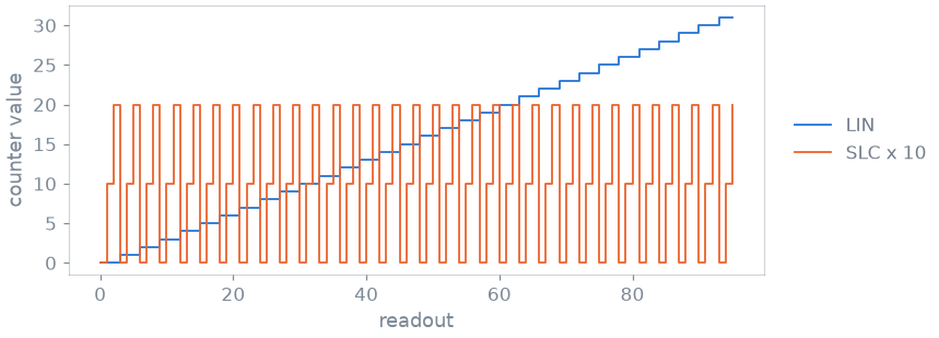
evaluate_labels() replays the label events in block order and, with evolution="adc", records every counter’s value at each readout. That is the table a reconstruction reads: for every readout, its line and its slice.

counters = seq.evaluate_labels(evolution="adc")
print(f"{len(counters['LIN'])} readouts")
print("LIN:", counters["LIN"][:9], "...")
print("SLC:", counters["SLC"][:9], "...")

96 readouts
LIN: [0 0 0 1 1 1 2 2 2] ...
SLC: [0 1 2 0 1 2 0 1 2] ...

LIN climbs one step every three readouts, SLC cycles through the three slices within each step. Each readout is fully described by these two counters, so a reconstruction can sort the stream into three k-spaces of 32 lines without knowing anything about how you wrote the loop.

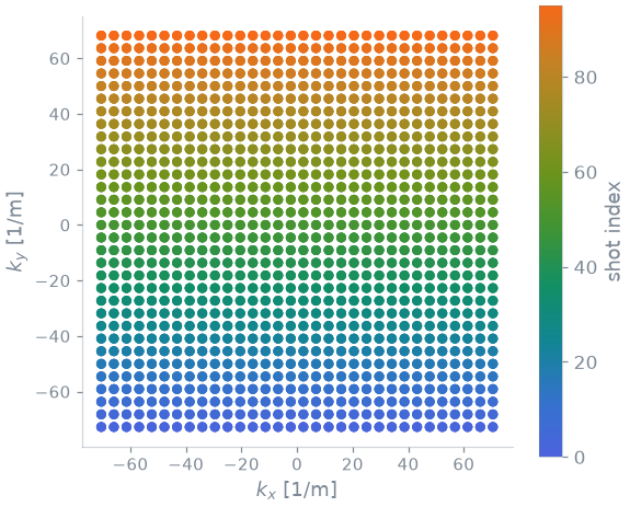
The same counters colour the k-space plot by acquisition order, read from the sequence:

pp.plot.plot_kspace(seq, plane="xy", color_by="order", show_trajectory=False)

pulserver turns these counters into the encoding counters of each MRD acquisition, which is how its reconstruction receives your labels.

Specification

What this lesson built, stated the way you would ask an agent for it:

Turn the lesson-3 spoiled gradient echo into a 3-slice acquisition
(slices at -10, 0 and 10 mm, 20 ms per slot, all slices of a line before
the next line) by setting the RF freq_offset to gz.amplitude * z and the
matching phase offset at the RF centre. Label every excitation block
with LIN and SLC using pypulseqpp.sequences.Labels, set the Name, FOV,
Matrix, SlicePositions and TR definitions, and read the counters back
per readout with evaluate_labels(evolution="adc").