Slice-selective excitation

A slice-selective pulse is played together with a selection gradient, so that only the spins within a slab of the chosen thickness are on resonance. Three numbers specify it: the flip angle, the slice thickness and the time-bandwidth product. This Tour designs excitations with the excitation module, simulates their slice profiles, and measures how the time-bandwidth product and the duration affect the profile, the selection gradient and the peak \(B_1\), and which combinations the gradient system admits.

The pulse and its selection gradient are not independent: the gradient places the pulse’s bandwidth across the slice,

\[G = \frac{\mathrm{TBW}}{\gamma\, T\, \Delta z} ,\]

so a shorter pulse at the same thickness and the same time-bandwidth product needs a proportionally stronger selection gradient and a proportionally larger \(B_1\). The gradient amplitude limit therefore bounds the two together.

Prerequisites: lessons 1 and 9 of the course.

The module concept is described in Sequence modules and functions.

import numpy as np

import pypulseqpp as pp
from pypulseqpp import sequences

#: Gyromagnetic ratio of the proton (Hz/T).
GAMMA = 42.576e6

THICKNESS = 5e-3
FLIP_ANGLE_DEG = 8.0

system = pp.Opts(
    max_grad=40.0,
    grad_unit="mT/m",
    max_slew=150.0,
    slew_unit="T/m/s",
    adc_dead_time=10e-6,
)

Excitation simulation

The excitation module designs the pulse, its selection gradient and the rephaser that unwinds the second half of the selection. Its sim_rf simulates the Bloch response of its pulse across off-resonance, which under a selection gradient of amplitude selection_amplitude is the slice profile, because a spin at position z is off-resonance by selection_amplitude * z.

def simulate(time_bw_product, duration_s):
    """Design one excitation and simulate the profile its pulse produces."""
    module = sequences.SpatialSelectiveExcitation(
        system,
        flip_angle_deg=FLIP_ANGLE_DEG,
        thickness_m=THICKNESS,
        duration_s=duration_s,
        time_bw_product=time_bw_product,
    )
    magnetisation, frequency = module.sim_rf()[1:3]
    profile = np.abs(magnetisation)
    return {
        "tbw": time_bw_product,
        "duration": duration_s,
        "gradient": module.selection_amplitude / GAMMA,
        "position": frequency / module.selection_amplitude,
        "profile": profile / profile.max(),
        "time": np.arange(module.rf.signal.size) * system.rf_raster_time,
        "envelope": np.abs(module.rf.signal),
        "peak_b1": float(np.abs(module.rf.signal).max()),
    }

Two numbers describe a profile: how far it takes to fall from the passband to the stopband, and how flat it is on either side of that transition.

def describe(simulated):
    """Transition width, passband ripple and stopband level of a profile."""
    position, profile = simulated["position"], simulated["profile"]
    edge = position > 0
    outward, falling = position[edge], profile[edge]

    def crosses(level):
        index = int(np.argmax(falling < level))
        return np.interp(
            level,
            [falling[index], falling[index - 1]],
            [outward[index], outward[index - 1]],
        )

    passband = profile[np.abs(position) < 0.35 * THICKNESS]
    stopband = profile[np.abs(position) > 1.5 * THICKNESS]
    return {
        **simulated,
        "transition": crosses(0.1) - crosses(0.9),
        "passband": float(passband.max() - passband.min()),
        "stopband": float(stopband.max()),
    }

The time-bandwidth product at a fixed duration

Every design below is 3 ms long and selects the same 5 mm. The pulse has more zero crossings as the time-bandwidth product rises, and the selection gradient rises with it so that the wider bandwidth still lands on the same slice.

PRODUCTS = (2.0, 4.0, 6.0, 8.0, 12.0)

by_product = [describe(simulate(product, 3e-3)) for product in PRODUCTS]

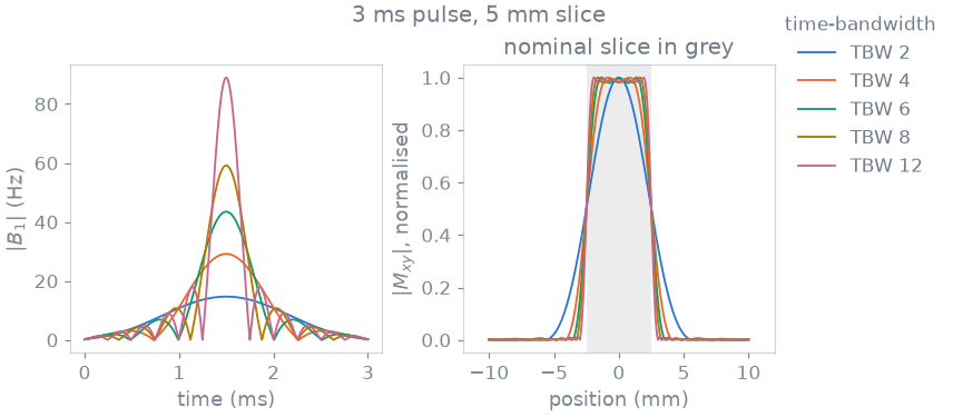
 tbw      gradient    transition    passband    stopband     peak B1
 2.0       3.03 mT/m      3.225 mm      0.2716      0.0041     14.7 Hz
 4.0       6.06 mT/m      1.823 mm      0.1429      0.0024     29.2 Hz
 6.0       9.21 mT/m      1.233 mm      0.0482      0.0015     43.5 Hz
 8.0      12.37 mT/m      0.928 mm      0.0201      0.0011     59.1 Hz
12.0      18.67 mT/m      0.619 mm      0.0143      0.0007     89.0 Hz

Above the smallest product the transition width falls close to inversely with it, so their product settles towards a figure set by the slice thickness rather than by the design. The passband ripple falls over the same range and the stopband stays below a percent throughout. The last column gives the corresponding increase in transmit amplitude: the peak \(B_1\) rises in proportion to the time-bandwidth product, because the same flip angle is delivered by an envelope with more structure in the same time.

The duration at a fixed time-bandwidth product

Varying duration at fixed time-bandwidth product separates slice-profile properties from gradient amplitude and peak \(B_1\) requirements.

DURATIONS = (1e-3, 2e-3, 3e-3, 5e-3, 8e-3)

by_duration = [describe(simulate(4.0, duration)) for duration in DURATIONS]

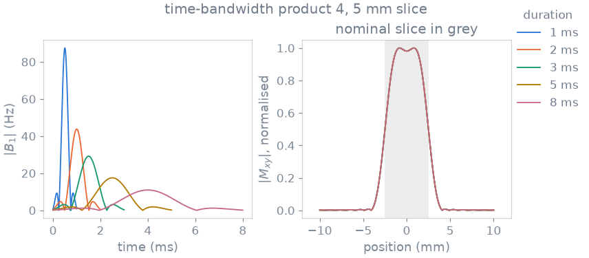
duration_ms      gradient    transition    passband    stopband     peak B1
       1.0      18.16 mT/m      1.823 mm      0.1459      0.0024     87.5 Hz
       2.0       9.08 mT/m      1.823 mm      0.1466      0.0024     43.8 Hz
       3.0       6.06 mT/m      1.823 mm      0.1429      0.0024     29.2 Hz
       5.0       3.63 mT/m      1.823 mm      0.1418      0.0024     17.5 Hz
       8.0       2.27 mT/m      1.823 mm      0.1442      0.0024     10.9 Hz

The five profiles lie on top of each other. The transition width is the same to three decimal places across an eightfold change of duration, and the small residual differences in the ripple follow the number of samples the pulse is written with: on a fixed RF raster a 1 ms envelope has an eighth of the samples of an 8 ms one. The duration sets the selection gradient and the peak \(B_1\), both of which scale as its reciprocal, and the time the repetition spends on the excitation.

Gradient amplitude limit

The two sweeps are two lines through one plane, and the amplitude limit cuts it along \(T = \mathrm{TBW} / (\gamma\, \Delta z\, G_\mathrm{max})\). A design above that line is realizable; one below it requires a selection gradient above the amplitude limit, and the module raises an error rather than widening the slice.

grid = []
for product in (2.0, 4.0, 6.0, 8.0, 12.0, 16.0):
    for duration in (0.3e-3, 0.5e-3, 1e-3, 2e-3, 3e-3, 5e-3):
        try:
            sequences.SpatialSelectiveExcitation(
                system,
                flip_angle_deg=FLIP_ANGLE_DEG,
                thickness_m=THICKNESS,
                duration_s=duration,
                time_bw_product=product,
            )
        except ValueError:
            feasible = False
        else:
            feasible = True
        grid.append({"tbw": product, "duration": duration, "feasible": feasible})

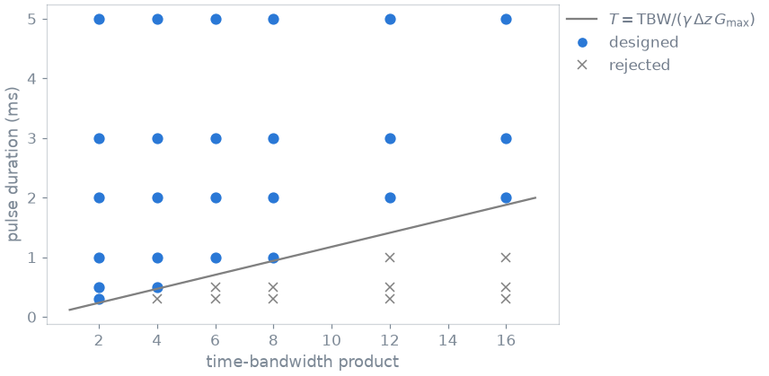
25 of 36 designs realizable, 11 rejected

The designs the module accepted are exactly those above the line. The bound is on the amplitude alone: changing the slew limit over the range a gradient system covers moves none of the points across it, because a lower slew rate lengthens the ramps on either side of the selection plateau, and hence the duration of the module, without changing the plateau amplitude.

The same plane read along its other axis gives the complementary statement: a sharper profile at a fixed slice thickness is available at any duration the gradient amplitude supports, and choosing between a long pulse and a strong gradient determines the echo time and the peak \(B_1\) rather than the profile.

Readout module

The sequence-module lesson of the course designed a stack-of-stars readout. LineReadout2D is the Cartesian counterpart: it takes the excitation’s events and a prescription (field of view, matrix, receiver bandwidth) and solves the readout, the phase encoding and the timing. With the echo time unset it uses the shortest echo time the prescription allows. The achieved receiver bandwidth is constrained by the rasters and can differ from the requested one; the module reports the achieved value.

FOV = 220e-3
MATRIX = 128

excitation = sequences.SpatialSelectiveExcitation(
    system, FLIP_ANGLE_DEG, THICKNESS, duration_s=3e-3, time_bw_product=4.0
)
readout = sequences.LineReadout2D(
    system,
    excitation.rf,
    excitation.gz,
    excitation.gz_reph,
    fov=(FOV, FOV),
    matrix=(MATRIX, MATRIX),
    te=None,
    readout_bandwidth_hz=250e3,
    spoiling_cycles=4.0,
)

print(
    f"echo time {1e3 * readout.echo_time:.3f} ms, "
    f"module {1e3 * readout.duration:.3f} ms\n"
    f"{readout.n_samples} samples at {readout.bandwidth_hz / 1e3:.1f} kHz, "
    f"echo on sample {readout.center_sample}, "
    f"line spacing {readout.delta_kx:.2f} 1/m"
)

echo time 2.800 ms, module 6.440 ms
128 samples at 100.0 kHz, echo on sample 64, line spacing 4.55 1/m

blocks is the module’s playout in order, as tuples of events. The loop adds them to a sequence and scales the phase-encode template to the line it is acquiring; here the largest step is played, and the pulse’s block is added first because the module is the readout half of the repetition.

seq = pp.Sequence(system=system)
seq.add_block(excitation.rf, excitation.gz)
for block in readout.blocks:
    seq.add_block(*block)

ok, errors = seq.check_timing()
print(f"timing {ok}, {seq.num_blocks} blocks, {1e3 * seq.duration()[0]:.3f} ms")

readout.paper_plot()

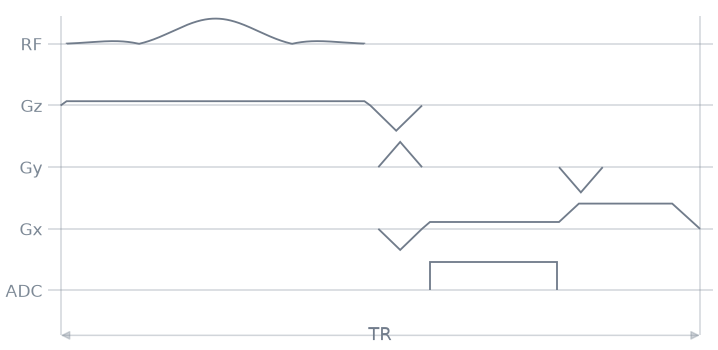
timing True, 5 blocks, 9.560 ms

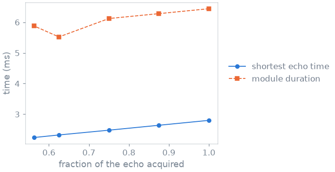
partial_echo is the fraction of the full echo acquired. It truncates the samples before the echo, and the shortest echo time follows: the samples that are no longer taken are the ones that stood between the excitation and the echo. You solve the module for each fraction:

FRACTIONS = (1.0, 0.875, 0.75, 0.625, 0.5625)


def solved(partial_echo=1.0, bandwidth_hz=250e3, **prescription):
    """One readout module, solved for the shortest echo time."""
    return sequences.LineReadout2D(
        system,
        excitation.rf,
        excitation.gz,
        excitation.gz_reph,
        fov=(FOV, FOV),
        matrix=(MATRIX, MATRIX),
        te=None,
        partial_echo=partial_echo,
        readout_bandwidth_hz=bandwidth_hz,
        spoiling_cycles=4.0,
        **prescription,
    )


partial = [
    {
        "fraction": fraction,
        "module": solved(partial_echo=fraction),
    }
    for fraction in FRACTIONS
]

partial echo   samples   echo on      achieved          TE      module
      1.0000       128        64      100.0 kHz    2.800 ms    6.440 ms
      0.8750       112        48      100.0 kHz    2.640 ms    6.280 ms
      0.7500        96        32      100.0 kHz    2.480 ms    6.120 ms
      0.6250        80        16      250.0 kHz    2.324 ms    5.520 ms
      0.5625        72         8      100.0 kHz    2.240 ms    5.880 ms

The sample the echo lands on moves with the fraction, and the echo time falls with it.

The achieved bandwidth is not the requested one at every fraction, nor the same at every fraction. A dwell time lies on the ADC raster and an acquisition window on the gradient raster, and whether a given dwell satisfies both depends on how many samples are taken: at 80 samples the requested 250 kHz lands on both rasters and is used, and at the neighbouring counts the fastest rate that does is 100 kHz. That is why the module duration does not fall monotonically while the echo time does, and why the module reports the achieved rate.

The module also plays echo trains (n_echoes, monopolar or bipolar with flyback); the trains themselves are built by hand in Multi-echo gradient echo and Echo planar imaging.

Specification

What this Tour built, stated the way you would ask an agent for it:

Using pypulseqpp sequence modules on a scanner with 40 mT/m and
150 T/m/s, design 8 degree slice-selective excitations of a 5 mm
slice with SpatialSelectiveExcitation. Simulate the slice profile
with sim_rf and report the transition width, passband ripple,
stopband level, selection gradient and peak B1, for time-bandwidth
products 2 to 12 at 3 ms and for durations 1 to 8 ms at a
time-bandwidth product of 4. Map which (product, duration) pairs
the amplitude limit admits. Then add a LineReadout2D for a 220 mm
FOV, 128x128 matrix at 250 kHz with the shortest TE, check the
timing, and tabulate the shortest TE for partial-echo fractions
1 to 0.5625.