Tensors and commands

This first lesson establishes how MR data from BART appear in Python: how a multichannel image and its k-space are laid out as tensors, which Fourier convention BART uses to go from k-space to the image, and how a BART command is called. Every later lesson relies on these conventions. A reconstruction that is off by a factor of \(\sqrt{N}\), or by a half-voxel shift from a misplaced k-space centre, is a consequence of misreading one of them.

bartorch runs BART inside the Python process. Every BART command is a function of bartorch.tools or of the bartorch namespace that takes and returns torch.Tensor objects, with no files and no subprocess in between. The lesson simulates a receive-array acquisition of BART’s analytical Shepp-Logan phantom, transforms it between image space and k-space, checks the transform against NumPy, and runs the same command once more through BART’s command line.

Learning objectives

• Relate a C-order tensor shape to BART’s dimension vector, and locate the receive-channel axis.

• Generate a phantom as an image, as coil images and as analytical k-space.

• State the centring and normalization of bartorch.fft(), and verify them against numpy.fft.fftn().

• Explain why analytically simulated k-space, truncated to the acquired matrix, reconstructs with Gibbs ringing.

• Call a BART command from Python, and the same command from its command line.

The next lesson, From k-space to image, reconstructs an undersampled acquisition with the functions introduced here.

import tempfile
from pathlib import Path

import numpy as np
import torch

import bartorch
import bartorch.tools as bt

SIZE = 128
COILS = 8

Array layout

BART stores an array in Fortran order and describes it by a dimension vector whose first entry varies fastest: readout (x), then the phase-encoding directions (y, z), then the receive channels in BART’s dimension 3, and further dimensions for sets of sensitivity maps, echoes, frames and so on. A tensor holding the same bytes in C order has the reversed shape, so no copy is needed between the two: a two-dimensional multichannel image is (coils, 1, y, x), with the singleton standing for BART’s z, and the readout direction is the last tensor axis. Data layout and conventions tabulates the layouts used throughout.

bartorch.tools.phantom() is BART’s phantom command. Without coils it returns the Shepp-Logan image; with coils it returns that image weighted by the complex receive sensitivities of BART’s analytical eight-channel head array, one image per channel.

image = bt.phantom(SIZE)
coil_images = bt.phantom(SIZE, coils=COILS)

print(f"image {tuple(image.shape)}, {image.dtype}")
print(f"coil images {tuple(coil_images.shape)}")
print(f"BART dimensions of the coil images {list(reversed(coil_images.shape))}")

image (128, 128), torch.complex64
coil images (8, 1, 128, 128)
BART dimensions of the coil images [128, 128, 1, 8]

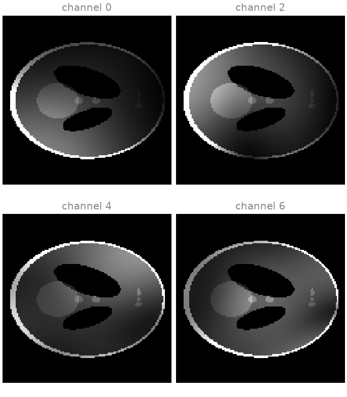
Each channel sees the object through its own sensitivity profile: bright near the coil element, dark on the opposite side of the head. The root sum of squares (RSS) over the channel axis, \(\sqrt{\sum_c |x_c|^2}\), is the standard magnitude combination of a receive array; it recovers the object with the residual shading of the summed sensitivity magnitudes. bartorch.rss() takes the channel axis as a tensor index, as every function of this package does, rather than as BART’s bitmask.

combined = bartorch.rss(coil_images, axes=(0,))
print(f"combined {tuple(combined.shape)}")

combined (1, 128, 128)

Fourier transform

The measured signal of a channel is the Fourier transform of its coil image, sampled on the k-space grid. bartorch.fft() is BART’s centred discrete transform: the k-space centre (DC) and the image centre are both at index n // 2, which is how k-space is displayed and how scanners deliver it. The transform is unnormalized unless unitary=True. For an even matrix size the centred transform equals NumPy’s transform between ifftshift and fftshift, which gives a reference computed outside BART.

kspace = bartorch.fft(coil_images, axes=(-2, -1), unitary=True)

shifted = np.fft.ifftshift(coil_images.numpy(), axes=(-2, -1))
reference = np.fft.fftshift(np.fft.fft2(shifted, norm="ortho"), axes=(-2, -1))

difference = np.abs(kspace.numpy() - reference).max() / np.abs(reference).max()
print(f"largest difference from numpy, relative to the peak: {difference:.1e}")

largest difference from numpy, relative to the peak: 1.7e-07

The difference is single-precision round-off. The unitary transform preserves the \(\ell_2\) norm (Parseval’s theorem), so white noise has the same standard deviation in k-space and in the image, a property the noise and SNR lessons rely on.

print(f"norm ratio image/k-space: {float(coil_images.norm() / kspace.norm()):.6f}")

norm ratio image/k-space: 1.000004

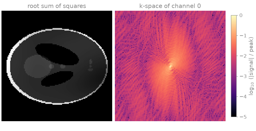
The k-space magnitude, drawn on a logarithmic scale, spans five orders of magnitude: the signal energy is concentrated at the centre, which sets the image contrast, while the periphery carries the edges and fine detail. This distribution is what variable-density undersampling exploits in the next lessons.

Analytical k-space

kspace=True evaluates the Fourier transform of the phantom’s ellipses analytically at the k-space sample positions, rather than transforming the sampled image. The two are different data. The continuous object has infinite spatial-frequency extent, and an acquisition of a finite matrix truncates it at \(\pm k_{\max}\); its inverse transform therefore carries Gibbs ringing, the oscillation next to every sharp edge that truncation artefacts produce on a scanner. The DFT of the sampled image, by contrast, reproduces that image exactly. Simulating data with the same discrete model the reconstruction inverts, the inverse crime [1], removes this discretization error from a simulation; analytical k-space retains it and is therefore the more realistic test data.

analytical = bt.phantom(SIZE, kspace=True)
truncated = bartorch.ifft(analytical, axes=(-2, -1))

error = float((truncated - image).norm() / image.norm())
print(f"relative difference from the sampled phantom: {error:.3f}")

relative difference from the sampled phantom: 0.218

• 
• 

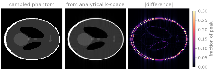
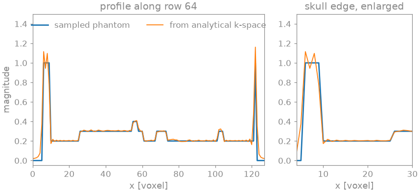
The difference map is largest at the ellipse boundaries and decays with distance from them. The profile through the centre of the phantom shows the ringing directly: the image from analytical k-space overshoots at every intensity step and oscillates with a period of about two voxels next to it. The unnormalized inverse transform is used here because phantom scales its k-space so that the unnormalized inverse returns the image’s intensities.

Commands and the command line

A function of bartorch.tools passes BART’s options as keyword arguments, under their long names or their single-letter flags, and reverses the dimension vector of each tensor it hands over. The bartorch console command takes BART’s own command lines and operates on CFL files, so a script written for the bart executable runs against the same library; bartorch.cli.main() runs one such command line in the current process. bartorch.io.writecfl() takes an array in BART’s order, which the transpose of a C-order array is.

with tempfile.TemporaryDirectory() as directory:
    source, target = str(Path(directory) / "coils"), str(Path(directory) / "kspace")
    bartorch.io.writecfl(source, coil_images.numpy().T)
    status = bartorch.cli.main(["fft", "-u", "3", source, target])
    from_files = torch.as_tensor(bartorch.cli.read(target))

print(f"exit status {status}, identical to bartorch.fft: {torch.equal(from_files, kspace)}")

exit status 0, identical to bartorch.fft: True

-u requests the unitary transform and 3 is BART’s bitmask for its dimensions 0 and 1 (readout and first phase-encoding direction), the last two tensor axes. The two routes run the same BART function on the same bytes, so the results are identical.

A BART command is not recorded by autograd: its result has no gradient with respect to its inputs. The operators of bartorch.linop and the solvers of bartorch.optim, introduced from Operators and solvers on, are differentiable. Interfaces and execution describes both routes.

References

[1]

Guerquin-Kern M, Lejeune L, Pruessmann KP, Unser M. Realistic analytical phantoms for parallel magnetic resonance imaging. IEEE Trans Med Imaging 31(3):626-636 (2012). https://doi.org/10.1109/TMI.2011.2174158