Off-resonance correction of spiral imaging

A spiral readout acquires each k-space radius at its own time, so a spin off resonance accrues a phase that varies over k-space: its image is blurred into a ring rather than shifted, as it would be along the readout of a Cartesian acquisition. With readouts of tens of milliseconds, the \(B_0\) inhomogeneity near air-tissue interfaces is enough to smear the temporal and orbitofrontal cortex over several voxels.

This example simulates an axial spiral acquisition of the head at 3 T in a \(B_0\) field computed from the magnetic susceptibility of the head, and corrects it with a known field map in two ways:

• by multifrequency interpolation (MFI) on the gridded image, bartorch.tools.deblur(), the method of Gadgetron’s spiral deblurring gadget;

• by a model-based reconstruction whose encoding operator includes the field map by time segmentation, bartorch.linop.FieldCorrected().

Learning objectives

• Relate the blurring of a spiral image to the off-resonance frequency and the readout duration.

• Describe a spiral readout by its time map \(t(|k|)\) and factorize its off-resonance transfer with fit_transfer().

• Choose the number of MFI demodulation frequencies.

• Set up a time-segmented model-based reconstruction, and recognise where it outperforms conjugate-phase methods such as MFI.

import math

import torch

import bartorch
import bartorch.tools as bt
from bartorch import linop, optim

Object and field map

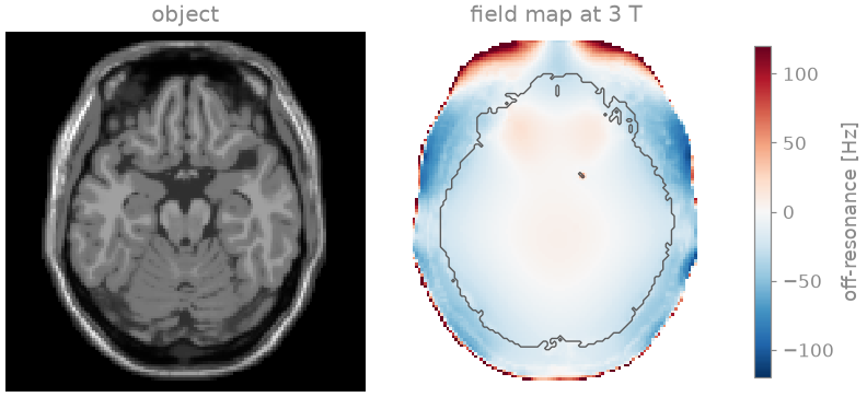
The object is an axial slice of the BrainWeb T1-weighted head [1] through the orbitofrontal cortex and the temporal lobes, 128 x 128 over a 220 mm field of view (1.7 mm in-plane). The field map is the \(B_0\) offset at 3 T produced by the susceptibility difference between air and tissue, \(\Delta\chi = 9.4\) ppm, computed in 3D with the dipole kernel and less a second-order shim fitted over the brain, rounded to 1 Hz, limited to \(\pm 150\) Hz, and set to zero outside the head, where a measured field map has no signal to be estimated from. The offsets are largest in the scalp; in the brain they reach about \(-40\) Hz in the lateral temporal lobes and \(+40\) Hz in the orbitofrontal cortex, a phase of about one cycle over the readout below.

SIZE, FOV_MM = 128, 220.0
for name, region in (("head", head), ("brain", brain)):
    values = field_map[region]
    print(f"field over the {name}: {float(values.min()):+.0f} to {float(values.max()):+.0f} Hz")

field over the head: -109 to +150 Hz
field over the brain: -41 to +44 Hz

The spiral readout

Four interleaves of an Archimedean spiral reach \(k_{max}\) at the Nyquist edge of the 128 matrix, each in a 24 ms readout of 6000 samples (4 µs dwell time). The interleaves are rotations of one arm by \(2\pi/4\), and the arm makes 16 turns, so the rings of the four interleaves together are one grid unit apart. Near the centre of k-space the angular velocity is limited by the slew rate and further out the trajectory speed by the gradient amplitude, which is modelled by the readout time \(t/T = (s^2 + 0.2\, s) / 1.2\) along the arm coordinate \(s = |k|/k_{max}\). The trajectory is in grid units.

INTERLEAVES, SAMPLES, READOUT_S = 4, 6000, 24e-3
TURNS = SIZE / 2 / INTERLEAVES

sample_time = torch.linspace(0.0, READOUT_S, SAMPLES, dtype=torch.float64)
arm = torch.sqrt(0.01 + 1.2 * sample_time / READOUT_S) - 0.1  # s(t)
angle = 2 * math.pi * TURNS * arm + 2 * math.pi * torch.arange(INTERLEAVES)[:, None] / INTERLEAVES
radius = SIZE / 2 * arm
trajectory = torch.stack(
    [radius * torch.cos(angle), radius * torch.sin(angle), torch.zeros_like(angle)], dim=-1
).float()
sample_time = sample_time.float()

The acquisition

A voxel at off-resonance frequency \(f\) contributes \(x(r)\, e^{-2\pi i k \cdot r}\, e^{2\pi i f\, t(k)}\) to the sample at \(k\). The acquisition is simulated exactly for the field map: each frequency’s part of the object is transformed with bartorch.nufft() and given the phase it accrues at each sample time. The reference is the same acquisition on resonance.

def acquire(field):
    samples = torch.zeros(INTERLEAVES, SAMPLES, 1, dtype=torch.complex64)
    for frequency in torch.unique(field[head]):
        part = image * ((field == frequency) & head)
        accrued = torch.polar(torch.ones(SAMPLES), 2 * math.pi * float(frequency) * sample_time)
        samples += bartorch.nufft(part, trajectory) * accrued[:, None]
    return samples


on_resonance = bartorch.nufft(image * head, trajectory)
off_resonance = acquire(field_map)

Gridding reconstruction

The images are reconstructed by the density-compensated adjoint NUFFT, with Pipe-Menon weights from bartorch.estimate_density(). A voxel off resonance by \(f\) is spread over a ring whose extent grows with the phase \(2\pi f T\) accrued by the end of the readout: one full cycle at \(f = 1/T \approx 42\) Hz.

density = bartorch.estimate_density(trajectory[..., :2].reshape(-1, 2), (SIZE, SIZE))
density = density.reshape(INTERLEAVES, SAMPLES, 1)


def grid(samples):
    return bartorch.nufft_adjoint(samples * density, trajectory, image_shape=(SIZE, SIZE))


reference = grid(on_resonance)
blurred = grid(off_resonance)

Multifrequency interpolation

Conjugate-phase reconstruction [2] demodulates each voxel at its own frequency, \(\hat x(r) = \sum_k w_k\, y_k\, e^{2\pi i k \cdot r} e^{-2\pi i f(r)\, t_k}\), which costs one transform per voxel. MFI [3] costs one transform per demodulation frequency: the transfer is approximated over the readout as \(e^{-2\pi i f t} \approx \sum_m a_m(f)\, e^{-2\pi i f_m t}\), the gridded image is demodulated at each \(f_m\) in k-space, and the demodulated images are combined voxel by voxel with the weights \(a_m(f(r))\).

ReadoutTiming tabulates the readout time as a function of \(|k|\) from one interleaf; the others are rotations of it and share it. fit_transfer() places the demodulation frequencies uniformly over the band of the field map and, unless given a number, takes the fewest that approximate the transfer to 1 % RMS, starting from \(\lceil 2.5\, f_{max}\, T \rceil\), the number Gadgetron’s MFIOperator uses.

timing = bt.ReadoutTiming.from_trajectory(trajectory[0, :, :2], duration=READOUT_S)
band = float(field_map[head].abs().max())
transfer = bt.fit_transfer(timing, band=band)
deblurred = bt.deblur(blurred, field_map, transfer)
print(
    f"band +-{band:.0f} Hz: {transfer.terms} demodulation frequencies, "
    f"RMS error of the transfer {transfer.error(timing):.1e}"
)

band +-150 Hz: 12 demodulation frequencies, RMS error of the transfer 6.2e-03

Time-segmented model-based reconstruction

The field map can instead be included in the encoding operator, \(y = \sum_l \operatorname{diag}(b_l)\, E\, \operatorname{diag}(c_l)\, x\), with \(E\) the NUFFT and the temporal and spatial coefficients \(b_l(t)\) and \(c_l(r)\) fitted to \(e^{2\pi i f(r) t}\) over the histogram of the field map [4]. FieldCorrected() builds the operator from the field map and the sample times, and CG solves the normal equations. Unlike conjugate-phase methods, it does not assume the field to be constant over the extent of the blurring.

E = linop.NoncartesianSense(
    torch.ones(1, SIZE, SIZE, dtype=torch.complex64), (SIZE, SIZE), traj=trajectory
)
A = linop.FieldCorrected(E, field_map, readout_time=sample_time, mask=head, segments=transfer.terms)
solve = optim.CG(maxiter=20)
model_based = solve(off_resonance[None, ..., 0], A)
model_uncorrected = solve(off_resonance[None, ..., 0], E)
model_reference = solve(on_resonance[None, ..., 0], E)

Results

The spiral samples a disc of radius \(k_{max}\), and the truncation of the object’s spectrum at its edge leaves ringing around the scalp in every reconstruction, on resonance too. The on-resonance reconstruction of each kind is therefore the best achievable with this readout, and each image is compared with the reconstruction of the same kind on resonance, as the normalized root-mean-square error (NRMSE) over the brain. The on-resonance reconstructions are compared with the object after a least-squares scaling.

def nrmse(estimate, truth):
    return float((estimate - truth)[brain].norm() / truth[brain].norm())


def scaled(estimate, truth):
    magnitude = estimate.abs()
    return magnitude * (magnitude * truth.abs())[brain].sum() / (magnitude**2)[brain].sum()


ground_truth = (image * head).abs()
for name, on_resonance_image in (("gridding", reference), ("CG", model_reference)):
    error = nrmse(scaled(on_resonance_image, ground_truth), ground_truth)
    print(f"{name + ', on resonance':23s} {error:.3f} against the object")
print(f"gridding, uncorrected   {nrmse(blurred, reference):.3f}")
print(f"gridding, MFI           {nrmse(deblurred, reference):.3f}")
print(f"CG, uncorrected         {nrmse(model_uncorrected, model_reference):.3f}")
print(f"CG, time-segmented      {nrmse(model_based, model_reference):.3f}")

gridding, on resonance  0.040 against the object
CG, on resonance        0.016 against the object
gridding, uncorrected   0.079
gridding, MFI           0.046
CG, uncorrected         0.088
CG, time-segmented      0.028

• 
• 
• 
• 
• 

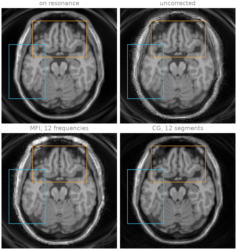
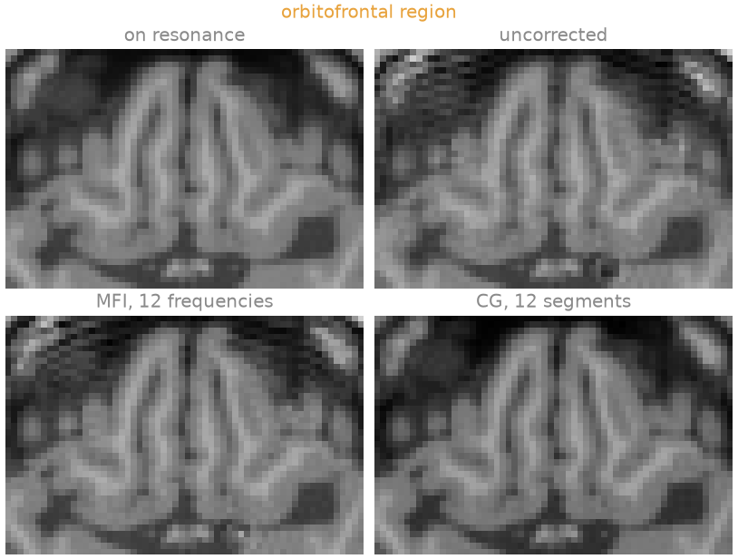
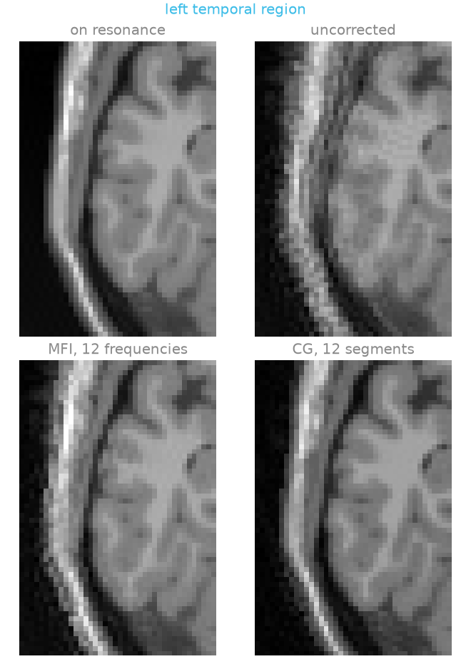
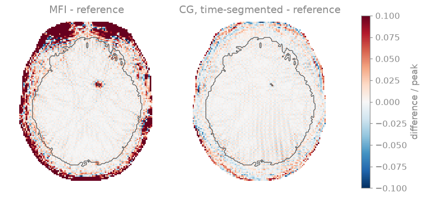
Uncorrected, the scalp, where the field is largest, is spread into a halo that overlaps the frontal and temporal cortex, and the cortex of the temporal lobes is smeared over a few voxels. MFI restores the brain to the accuracy of exact conjugate-phase reconstruction, one demodulation per distinct frequency of the field map. Its residual is concentrated in the scalp, where the field changes by tens of hertz within the extent of a voxel’s blurring ring: conjugate phase assumes the field constant over that extent, and where it is not, the demodulation leaves an intensity error. The time-segmented reconstruction models the phase of each voxel up to the segmentation error and removes that residual too, at the cost of an iterative solve with one NUFFT pair per segment and iteration, against one FFT pair per demodulation frequency for MFI.

The number of demodulation frequencies

The MFI approximation is poor until the demodulation frequencies are about \(1/T\) apart. The rows below give, for the band of this field map, the RMS error of the transfer, the largest \(\sum_m |a_m(f)|\) – the factor by which noise and residual error are amplified – and the NRMSE of the corrected image over the brain.

print(f"{'terms':>5}  {'transfer':>8}  {'sum|a|':>6}  {'brain NRMSE':>11}")
for terms in (9, 13, 17, 21, 25):
    trial = bt.fit_transfer(timing, band=band, terms=terms)
    corrected = bt.deblur(blurred, field_map, trial)
    print(
        f"{terms:5d}  {trial.error(timing):8.1e}  {trial.amplification:6.1f}  "
        f"{nrmse(corrected, reference):11.3f}"
    )

terms  transfer  sum|a|  brain NRMSE
    9   1.6e-01     2.3        0.177
   13   1.9e-03    14.8        0.046
   17   8.7e-06   191.6        0.046
   21   1.7e-08  2853.1        0.046
   25   3.0e-10  1777.4        0.046

Beyond the point where the transfer error is small, more frequencies leave the image unchanged and raise the amplification. Gadgetron’s gpuSpiralDeblurGadget sets the band from the echo spacing of its field map, \(f_{max} = 1.2 / (2\,\Delta TE)\), estimates the field map from a low-pass filtered two-echo spiral, and applies MFI with \(\lceil 2.5\, f_{max}\, T \rceil\) frequencies. Here the field map is known; in practice its own error and smoothing limit both corrections.

References

[1]

Collins DL, Zijdenbos AP, Kollokian V, Sled JG, Kabani NJ, Holmes CJ, Evans AC. Design and construction of a realistic digital brain phantom. IEEE Trans Med Imaging 17(3):463-468 (1998). https://doi.org/10.1109/42.712135

[2]

Noll DC, Meyer CH, Pauly JM, Nishimura DG, Macovski A. A homogeneity correction method for magnetic resonance imaging with time-varying gradients. IEEE Trans Med Imaging 10(4):629-637 (1991). https://doi.org/10.1109/42.108599

[3]

Man LC, Pauly JM, Macovski A. Multifrequency interpolation for fast off-resonance correction. Magn Reson Med 37(5):785-792 (1997). https://doi.org/10.1002/mrm.1910370523

[4]

Sutton BP, Noll DC, Fessler JA. Fast, iterative image reconstruction for MRI in the presence of field inhomogeneities. IEEE Trans Med Imaging 22(2):178-188 (2003). https://doi.org/10.1109/TMI.2002.808360