Parameter maps from scanner images

This lesson estimates a \(T_2\) map from the magnitude images a scanner exports, without access to the raw data: a multi-echo spin-echo series is read from DICOM, the decay is fitted voxel by voxel, and the map is written back as a DICOM series of the same study and as a NIfTI volume. The aim is to show the geometry and the acquisition timings passing from the scanner’s files to the fit and on to the output unchanged, so that the map overlays the images it was computed from.

Many protocols export each echo of a multi-echo acquisition, or each inversion time of an inversion-recovery experiment, as a DICOM series of its own. bartorch.io.read_dicom() reads several series as one, sorts the images into contrasts by their echo, inversion and repetition times, and returns those times with the images: they are the sampling points of the signal model. The images and the model are then those of Parameter maps straight from k-space, minus the Fourier encoding: the fit of bartorch.apps.mobafit() is Gauss-Newton on the signal equation alone.

A magnitude image is not Gaussian where the signal is small: its noise is Rician and has a positive floor, which a decay model fitted to it reads as a longer \(T_2\). mobafit() with magnitude=True fits the magnitude of the model to the magnitude of the data, which removes the phase from the problem but not the floor; the echoes here stay above it.

The input series is simulated in a hidden cell and written to a temporary directory, standing in for an export from the scanner.

Learning objectives

• Read a multi-echo series stored as one DICOM series per echo, with its echo times and its voxel-to-world affine.

• Fit bartorch.nlop.MultiEcho to magnitude images with bartorch.apps.mobafit().

• Write the map as a DICOM series of the same study, and as NIfTI, in the geometry of the input.

It follows Parameter maps straight from k-space. The next section, Plug-and-play denoisers, replaces a specified regularizer with a learned denoiser.

import tempfile
from pathlib import Path

import numpy as np
import torch

from bartorch import apps, io, nlop

Reading the series

The export holds one series per echo, numbered 101 to 108. Asked for all of them, read_dicom() returns the images as (contrasts, slices, rows, columns) in order of echo time, the echo times themselves in milliseconds, and the affine from voxel indices to RAS millimetres; every echo has to cover the same slices.

echoes = io.read_dicom(scanner, series=range(101, 109))
te = echoes.timings["echo_time"]

print(f"images {tuple(echoes.image.shape)}, TE {te.tolist()} ms")
print("voxel size", " x ".join(f"{v:.1f}" for v in echoes.affine[:3, :3].norm(dim=0)), "mm")

images (8, 1, 128, 128), TE [10.0, 20.0, 30.0, 40.0, 50.0, 60.0, 70.0, 80.0] ms
voxel size 1.7 x 1.7 x 4.0 mm

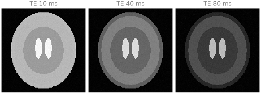
The images of three of the echoes, on one window: the cerebrospinal fluid in the ventricles, with the longest \(T_2\), keeps its signal across the train while the scalp fat loses most of it.

Fitting the decay

bartorch.nlop.MultiEcho is built on the echo times the files state and on the in-plane shape of the slice. The fit is voxel by voxel, so the slice axis is dropped here; a volume is fitted the same way with the model built on (slices, rows, columns). DICOM stores intensities in arbitrary units; the fit scales the echoes to unit peak and returns the amplitude in the units of the files.

images = echoes.image[:, 0].to(torch.complex64)
M = nlop.MultiEcho(te.tolist(), tuple(images.shape[1:]))
maps = apps.mobafit(images, M, magnitude=True, T2=80.0)
t2 = torch.where(images[0].abs() > 0.05 * images.abs().max(), maps["T2"], torch.zeros(()))

for (region, truth, _), name in zip(compartments, ("fat", "grey matter", "white matter", "CSF")):
    inner = torch.from_numpy(region)
    print(f"{name:>13}: T2 {float(t2[inner].median()):6.1f} ms against {truth:5.1f} ms")

         fat: T2   45.0 ms against  45.0 ms
 grey matter: T2   85.0 ms against  85.0 ms
white matter: T2   70.0 ms against  70.0 ms
         CSF: T2  250.1 ms against 250.0 ms

Writing the map

The map goes back to DICOM as a series of the same study: the first echo’s dataset lends its patient, study and frame of reference, and the series gets a number and a description of its own. ImageType marks it as derived. NIfTI stores the same affine, which is what a registration or a segmentation package reads.

output = Path(tempfile.mkdtemp())
io.write_dicom(
    output / "t2-map",
    t2,
    echoes.affine,
    header=echoes.header,
    SeriesNumber=201,
    SeriesDescription="T2 map",
    ImageType=["DERIVED", "PRIMARY", "T2 MAP"],
)
io.write_nifti(output / "t2-map.nii.gz", t2, echoes.affine)

written = io.read_dicom(output / "t2-map")
same_study = written.header.StudyInstanceUID == echoes.header.StudyInstanceUID
print(f"patient {written.header.PatientID}, same study {same_study}")
print(f"largest affine difference {float((written.affine - echoes.affine).abs().max()):.1e} mm")

patient P0001, same study True
largest affine difference 2.0e-06 mm

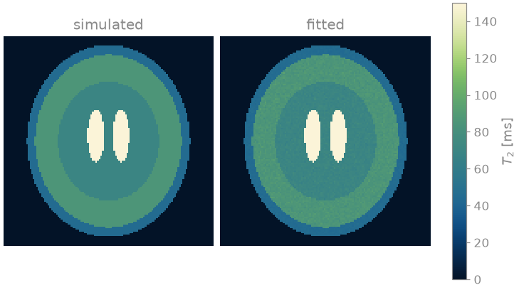
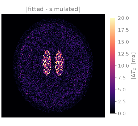
The map read back from the DICOM series beside the \(T_2\) the images were simulated with, and the difference between them. The error is largest in the cerebrospinal fluid, where eight echoes over 80 ms sample only the start of a 250 ms decay.

• 
•