Networks for complex volumes

Aim. Train a 3D convolutional denoiser on patches of a complex, multi-contrast brain volume, apply it to a whole volume of another subject patch by patch, as it would run on a scanner GPU too small for the volume, and check that the patch boundaries leave no visible seams.

The networks of the previous lessons denoise a single complex 2D slice. The data a learned reconstruction is most needed for are larger: a 3D volume of several contrasts, of subspace coefficients in MR fingerprinting, or of the frames of a cine. Three things change. The contrasts are denoised jointly, as channels of one image, so that the network can use the anatomy they share; their signal levels differ, so they are balanced before the network sees them. The volume does not fit the network’s activations in GPU memory, so the network is trained on patches and applied patch by patch. And a network applied on a fixed grid of patches leaves seams at the patch boundaries, which a random offset of the grid averages out.

Learning objectives

• Build a 3D bartorch.learning.UNet for complex multi-contrast images with bartorch.learning.ComplexNet, and balance the contrasts by whitening.

• Train it on patches drawn by torchio, with augmentations that preserve the complex MR signal.

• Apply it to a whole volume with bartorch.learning.Patchwise, and average the seams out with bartorch.learning.moments().

• Compare the size of spatial and spatiotemporal networks.

It follows MoDL, on BART’s ADMM. The next lesson, Staged training of an unrolled network, trains an unrolled network in stages.

import csv
import logging
from pathlib import Path

import brainweb_dl
import lightning
import numpy as np
import torch
import torchio as tio
from brainweb_dl import get_mri
from torch.utils.data import DataLoader

from bartorch import learning

SIZE = 64
PATCH = 32
NOISE = 0.06

_ = torch.manual_seed(0)

A multi-contrast complex volume

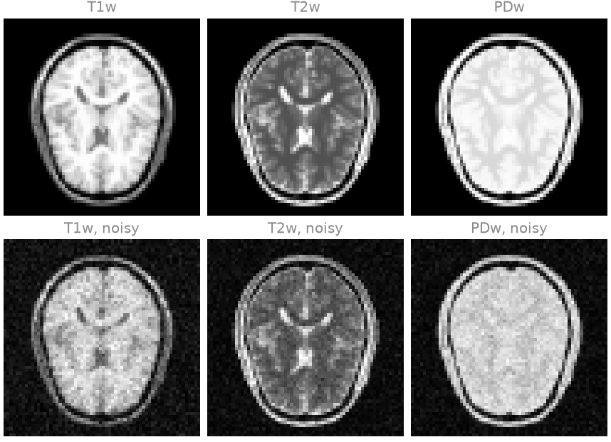
Three spin-echo contrasts of a BrainWeb subject – \(T_1\)-weighted (TR 600 ms, TE 12 ms), \(T_2\)-weighted (TR 4000 ms, TE 100 ms) and proton-density-weighted (TR 4000 ms, TE 12 ms) – on a \(64^3\) grid, each with its own smooth background phase, as a (3, z, y, x) complex tensor. Each voxel’s signal is the sum of the spin-echo signals of the tissues it contains. Subject 0 is the training volume and subject 4 the test volume. Complex Gaussian noise of 6 per cent of each contrast’s peak gives the test volume an SNR typical of a fast high-resolution scan.

train_volume = brain_volume(subject=0)
test_volume = brain_volume(subject=4)
noisy = test_volume + NOISE * torch.randn_like(test_volume)
print(f"test volume {tuple(test_volume.shape)}, {test_volume.dtype}")

test volume (3, 64, 64, 64), torch.complex64

The network

UNet is a residual U-Net whose last convolution starts at zero, so that the untrained network returns its input. ComplexNet lays the three complex contrasts out as its six real channels – the real parts, then the imaginary parts – and lays its output back out as complex contrasts. With normalize="whiten" it subtracts each channel’s mean and multiplies by the inverse square root of the channels’ covariance before the call, and undoes both after it, so that the network sees uncorrelated channels of unit variance whatever the relative energy of the contrasts.

net = learning.UNet(6, spatial=3, widths=(8, 16, 32))
denoiser = learning.ComplexNet(net, spatial=3, channels=1, normalize="whiten")
weights = sum(p.numel() for p in net.parameters())
print(f"{weights} weights, {4 * weights / 1e6:.2f} MB in single precision")

with torch.no_grad():
    print(
        "untrained network returns its input:",
        torch.allclose(denoiser(noisy[None])[0], noisy, atol=1e-5),
    )

136942 weights, 0.55 MB in single precision
untrained network returns its input: True

Patches and augmentation

torchio holds the training volume as a torchio.ScalarImage of real channels (as_real()) and draws \(32^3\) patches from it through a torchio.Queue. The augmentations are those that map one MR image to another the acquisition could have produced: a flip, and RandomGain, a receiver gain and global phase shared by the contrasts. An intensity transform applied to the real and imaginary channels separately, such as a gamma correction, would produce a signal no acquisition can. The global phase is varied over a limited range: a network trained over every phase must learn to commute with a rotation of its real and imaginary channels, which takes more training than this lesson runs.

Each patch becomes a training pair when a new draw of noise is added to it, so the network sees a different noise realization at every epoch.

subject = tio.Subject(image=tio.ScalarImage(tensor=learning.as_real(train_volume).flatten(0, 1)))
augment = tio.Compose(
    [tio.RandomFlip(axes=(0, 1, 2)), learning.RandomGain(phase=0.3, log_scale=0.2)]
)
queue = tio.Queue(
    tio.SubjectsDataset([subject], transform=augment),
    max_length=64,
    samples_per_volume=32,
    sampler=tio.UniformSampler(PATCH),
    num_workers=0,
)


def pairs(patches):
    made = []
    for patch in patches:
        clean = learning.as_complex(patch["image"][tio.DATA].unflatten(0, (2, 3)))
        made.append({"input": clean + NOISE * torch.randn_like(clean), "target": clean})
    return made


validation = [{"input": noisy, "target": test_volume}]
trainer = lightning.Trainer(
    max_epochs=30,
    accelerator="cpu",
    logger=False,
    enable_checkpointing=False,
    enable_model_summary=False,
    enable_progress_bar=False,
)
trainer.fit(
    learning.Reconstruction(denoiser, "denoiser", lr=2e-3),
    DataLoader(queue, batch_size=4, collate_fn=pairs),
    DataLoader(validation, batch_size=1, collate_fn=list),
)

/opt/hostedtoolcache/Python/3.12.14/x64/lib/python3.12/site-packages/lightning/pytorch/utilities/_pytree.py:21: `isinstance(treespec, LeafSpec)` is deprecated, use `isinstance(treespec, TreeSpec) and treespec.is_leaf()` instead.
/opt/hostedtoolcache/Python/3.12.14/x64/lib/python3.12/site-packages/lightning/pytorch/trainer/connectors/data_connector.py:434: The 'val_dataloader' does not have many workers which may be a bottleneck. Consider increasing the value of the `num_workers` argument` to `num_workers=3` in the `DataLoader` to improve performance.
/opt/hostedtoolcache/Python/3.12.14/x64/lib/python3.12/site-packages/lightning/pytorch/trainer/connectors/data_connector.py:434: The 'train_dataloader' does not have many workers which may be a bottleneck. Consider increasing the value of the `num_workers` argument` to `num_workers=3` in the `DataLoader` to improve performance.

Applying the network patch by patch

Patchwise keeps the volume in host memory and sends it to the network’s device a few patches at a time, runs the network there in mixed precision, and assembles the result on the host. On a GPU only the network and batch patches are resident, so a volume larger than the GPU memory – a whole-brain fingerprinting series on a scanner’s 16 GB GPU – is denoised by a network trained on patches of it. At inference the copies of one group of patches overlap the computation on the previous one. Here, on the host, the whole volume is also small enough to be denoised in one call, which is the reference the patchwise result is compared with.

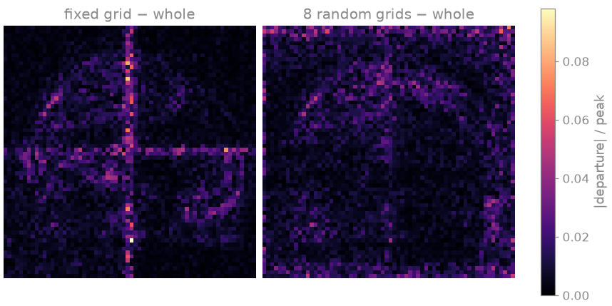
A U-Net is not translation invariant at a patch boundary: its receptive field extends past the patch, where it sees zeros rather than the neighbouring voxels. On a fixed grid of patches the errors fall along the same planes every time. With shift=True, the grid is offset at random at every call, and averaging a few calls with moments() spreads the boundary errors across the volume.

whole_net = learning.ComplexNet(net, spatial=3, channels=1, normalize="whiten")
fixed = learning.ComplexNet(
    learning.Patchwise(net, (PATCH,) * 3, shift=False), spatial=3, channels=1, normalize="whiten"
)
shifted = learning.ComplexNet(
    learning.Patchwise(net, (PATCH,) * 3, shift=True), spatial=3, channels=1, normalize="whiten"
)

with torch.no_grad():
    whole = whole_net(noisy[None])[0]
    grid = fixed(noisy[None])[0]
    averaged, spread = learning.moments(lambda: shifted(noisy[None])[0], samples=8)


def error(made):
    return float((made - test_volume).norm() / test_volume.norm())


print(f"noisy                  relative error {error(noisy):.4f}")
for name, made in (("whole volume", whole), ("fixed grid", grid), ("8 random grids", averaged)):
    print(
        f"{name:<22} relative error {error(made):.4f}, "
        f"departure from the whole volume {float((made - whole).norm() / whole.norm()):.4f}"
    )

• 
• 
• 

noisy                  relative error 0.1850
whole volume           relative error 0.1147, departure from the whole volume 0.0000
fixed grid             relative error 0.1169, departure from the whole volume 0.0321
8 random grids         relative error 0.1219, departure from the whole volume 0.0487

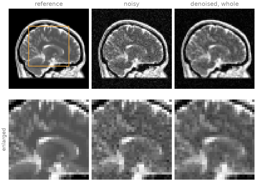
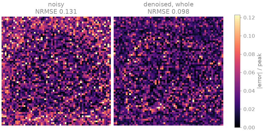
The network, 0.14 million weights trained for a few minutes on patches of one head, removes a third or more of the noise of the other head’s volume without blurring the white-matter tracts or the corpus callosum; a real training set and a wider network remove more.

The departure of the fixed grid from the whole-volume result lies on the planes between patches – the seams – and on the same planes at every call. A shifted grid covers the volume with one more patch along each axis and so has more boundaries, and a single call departs further from the whole-volume result; but the boundaries move from call to call, and the average of eight calls spreads the departure over the volume instead of concentrating it on planes, where it would read as an anatomical edge. Inside an iteration, which applies the denoiser once per step, one shifted grid per call is enough: no plane receives the boundary error at every step. The variance moments() returns is a map of how much the result depends on where the patches fall, one of the spreads of Uncertainty estimation.

Size of the network

The weights determine the storage footprint and, with the patch size, the memory of a call. The default widths of UNet, (32, 64, 128, 256), give a three-dimensional network of a few million weights. A series of frames – a cine, a functional run – is taken with frames=True: the network then convolves each frame spatially and the frames with a separate one-dimensional convolution, and never downsamples the frame axis; periodic=True pads it circularly, which suits a cardiac cycle. This factorization costs few weights beyond the spatial network.

for name, candidate in (
    ("3D, widths (8, 16, 32)", net),
    ("3D, default widths", learning.UNet(6, spatial=3)),
    ("3D + frames, default widths", learning.UNet(6, spatial=3, frames=True, periodic=True)),
):
    count = sum(p.numel() for p in candidate.parameters())
    print(f"{name:<28} {count / 1e6:5.2f} M weights, {2 * count / 1e6:5.1f} MB in half precision")

frames = torch.randn(1, 6, 10, 16, 16, 16)
cine = learning.UNet(6, spatial=3, widths=(8, 16), frames=True, periodic=True)
print("(n, channels, frames, z, y, x):", tuple(cine(frames).shape))

3D, widths (8, 16, 32)        0.14 M weights,   0.3 MB in half precision
3D, default widths            8.82 M weights,  17.6 MB in half precision
3D + frames, default widths   9.48 M weights,  19.0 MB in half precision
(n, channels, frames, z, y, x): (1, 6, 10, 16, 16, 16)