Parameter maps straight from k-space

This lesson estimates a \(T_2\) map from an undersampled multi-echo spin-echo acquisition in two ways, and compares them: reconstructing an image per echo and fitting the decay voxel by voxel afterwards, and fitting the signal model directly to the k-space data. The aim is to show why the second, model-based reconstruction, tolerates undersampling that ruins the first.

In a multi-echo spin-echo (CPMG) acquisition the signal of each voxel decays from echo to echo as \(M_0 \exp(-\mathrm{TE}/T_2)\). Undersampling each echo shortens the scan, but a reconstruction of each echo on its own is an ill-posed problem, and its aliasing and noise differ from echo to echo; a voxelwise fit cannot tell them apart from decay, and carries them into the map. The model-based approach [1] [2] puts the signal model inside the forward operator,

\[y_{c,e} = P_e F \, (S_c \cdot M_e(\theta)),\]

where \(P_e\) is the sampling pattern of echo \(e\), \(F\) the Fourier transform, \(S_c\) the sensitivity of coil \(c\), \(M\) the signal model and \(\theta\) the parameter maps, and solves for \(\theta\) from the k-space data of all echoes at once. The unknowns are then three real maps rather than eight complex images, and every echo constrains all of them. The operator is nonlinear in \(\theta\), so the problem is solved by the iteratively regularized Gauss-Newton method of Nonlinear inversion, over a different model.

The model here is bartorch.nlop.MultiEcho, a TorchSim simulator as a BART nonlinear operator. The phantom and the coil sensitivities are built as in From k-space to image; the cell that does it is hidden on this page and present in the script this page can be downloaded as.

Learning objectives

• Represent a relaxation model as a TorchSim-backed bartorch.nlop.SignalModel.

• Fit it to reconstructed echo images, and directly to k-space by composing it with the encoding, with bartorch.nlop.IRGNM.

• Run the same fits through bartorch.apps.mobafit() and bartorch.apps.moba().

• Explain, from the echo images and the error maps, why the model-based fit is more accurate at the same undersampling.

It follows Subspace-constrained T1 mapping, and Parameter maps from scanner images fits the same model to images read from DICOM.

import csv
import time
from pathlib import Path

import brainweb_dl
import numpy as np
import torch
from brainweb_dl import get_mri

import bartorch
import bartorch.tools as bt
from bartorch import apps, linop, nlop, optim

SIZE = 64
COILS = 8
ECHOES = 8
ACCELERATION = 4

ECHO_TIMES = torch.tensor([12.5 * (echo + 1) for echo in range(ECHOES)])  # ms

Phantom

The \(T_2\) of each tissue class from the BrainWeb table, combined by membership, and the echo images from the mono-exponential decay \(M_0 \exp(-\mathrm{TE}/T_2)\) written out here rather than taken from the model that will be fitted.

contrasts = (amplitude[None] * torch.exp(-ECHO_TIMES[:, None, None] / t2[None])).to(torch.complex64)

Acquisition

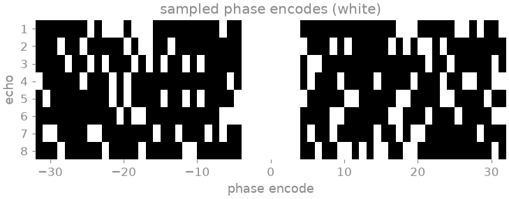
Eight echoes at an echo spacing of 12.5 ms, each sampled at a quarter of the phase encodes (\(R = 4\)) around eight fully sampled central lines, with a different random draw per echo, so that the missing phase encodes differ between echoes. The echoes are a batch of the encoding rather than an axis inside it: the sensitivities and the transform are shared, and only the pattern differs, so the operator is the Cartesian SENSE encoding of Operators and solvers with the pattern of each echo applied to its samples.

encoding = linop.CartesianSense(sensitivities, (ECHOES, SIZE, SIZE), ndim=2)
E = linop.Diagonal(lines.to(torch.complex64), encoding.oshape) @ encoding

measured = bt.noise(E(contrasts), n=1e-6, s=9)
data = measured / float(E.H(measured).abs().max())

print(f"{E.ishape} -> {E.oshape}")

(8, 64, 64) -> (8, 8, 64, 64)

The signal model

bartorch.nlop.MultiEcho maps parameter maps to one image per echo. Its unknowns are \(T_2\) and a complex amplitude, carried as three real maps in a bounded parameterisation rather than in their own units, so initial() builds a starting point from values and split() reads the fit back.

M = nlop.MultiEcho([float(te) for te in ECHO_TIMES], (SIZE, SIZE))
start = M.initial(T2=80.0)

print(f"unknowns {M.names}: {M.ishapes[0]} -> {M.oshapes[0]}")

unknowns ('T2', 'amplitude.real', 'amplitude.imag'): (3, 64, 64) -> (8, 64, 64)

Two routes

The first reconstructs the echo images by conjugate gradients on the SENSE normal equations and fits the model to them voxel by voxel, which is what bartorch.apps.mobafit() does given the images. The second composes the model with the encoding and fits the k-space with bartorch.nlop.IRGNM. Both are Gauss-Newton loops of the same number of steps and differ only in the forward operator that maps the unknowns to the data.

STEPS = 20

start_time = time.perf_counter()
images = optim.CG(maxiter=40)(data, E)
two_step = apps.mobafit(images, M, iterations=STEPS, T2=80.0)
print(f"reconstruct, then fit:     {time.perf_counter() - start_time:5.1f} s")

start_time = time.perf_counter()
model_based = nlop.IRGNM(iterations=STEPS, cg_maxiter=100, cg_tol=0.1)(data, E @ M, x0=start)
print(f"model inside the operator: {time.perf_counter() - start_time:5.1f} s")

/opt/hostedtoolcache/Python/3.12.14/x64/lib/python3.12/site-packages/torch/jit/_script.py:1491: FutureWarning: `torch.jit.script` is deprecated. Please switch to `torch.compile` or `torch.export`.
  warnings.warn(
reconstruct, then fit:       3.8 s
model inside the operator:   9.6 s

E @ M composes a linear operator with a nonlinear one; the derivative of the composition at a point is the encoding applied to the derivative of the model, which is the derivative a Gauss-Newton step requires.

The echo images of the first route show what its fit is given. They are compared here with the fully sampled echo images of the phantom.

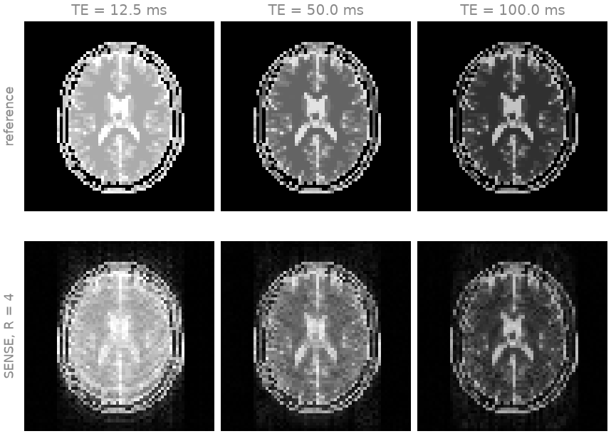
Each reconstructed echo carries residual aliasing and noise, which differ from echo to echo because each echo has its own sampling pattern. At the later echoes the signal has decayed and the relative error grows, so the late echoes, which determine \(T_2\) most, are also the least accurate.

bartorch.apps.moba() assembles the model-based composition from the k-space, the model, the sensitivities and the sampling pattern, and returns the maps in their own units. It scales the data by the rule of bartorch.optim.data_scaling() and regularizes each step towards the starting maps rather than towards zero, so its result is not identical to the fit above.

start_time = time.perf_counter()
one_call = apps.moba(measured, M, sensitivities, pattern=lines, iterations=STEPS, T2=80.0)
print(f"apps.moba:                 {time.perf_counter() - start_time:5.1f} s")

estimates = {
    "two-step": two_step["T2"],
    "model-based": M.split(model_based)["T2"],
    "apps.moba": one_call["T2"],
}

for name, estimate in estimates.items():
    error = float((estimate[support] - t2[support]).norm() / t2[support].norm())
    median = float(estimate[support].median())
    print(f"{name:>22}  median {median:5.1f} ms   relative error {error:.3f}")

print(f"{'phantom':>22}  median {float(t2[support].median()):5.1f} ms")

apps.moba:                  10.3 s
              two-step  median  86.1 ms   relative error 0.477
           model-based  median  81.5 ms   relative error 0.007
             apps.moba  median  81.3 ms   relative error 0.057
               phantom  median  81.5 ms

• 
• 

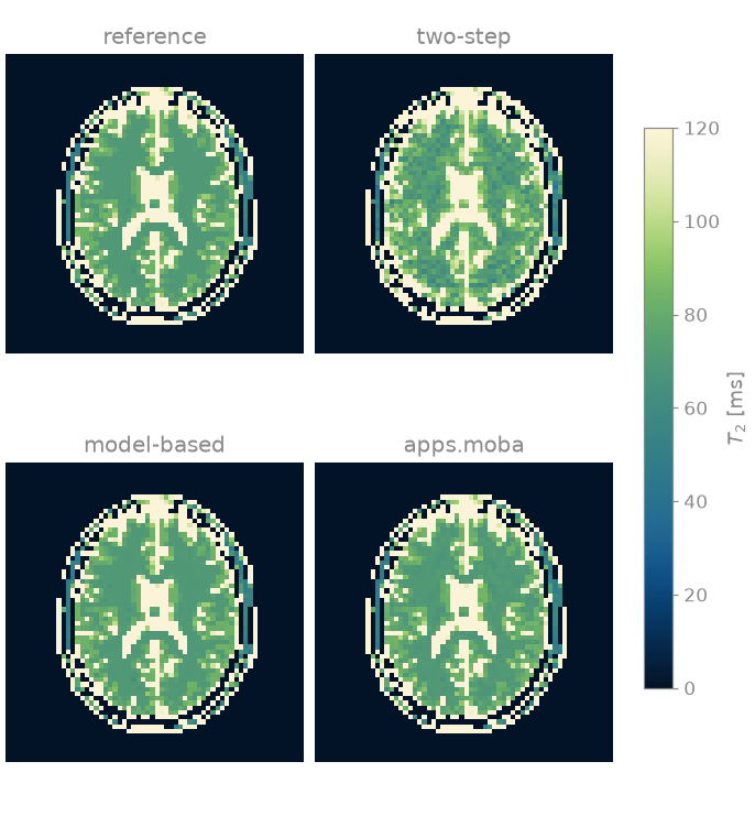
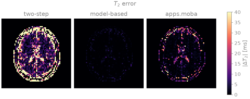
The two-step \(T_2\) map is dominated by the errors of the echo images: a voxelwise fit cannot distinguish residual aliasing from decay, and in voxels where a late echo is too bright or too dark the fitted \(T_2\) is far off. The model-based fits reach a much lower error from the same data, since the model admits only images that decay exponentially from echo to echo, and the aliasing of eight different sampling patterns is not such an image. The fit inside the operator reproduces the phantom almost exactly, because every voxel of the phantom decays with a single \(T_2\), as the model assumes; a measured voxel holding two tissues decays with two, and a single exponential cannot represent it. bartorch.apps.moba() regularizes each Gauss-Newton step towards the starting maps, and its residual error is largest where \(T_2\) is farthest from the starting value of 80 ms: in cerebrospinal fluid and the scalp. The maps are drawn with the navia colormap [3] in a window that spans white and grey matter.

Since the maps are the solver’s unknowns, a regularizer passed to the linearized problem – the inner solver of bartorch.apps.moba() – penalizes the maps rather than the echo images. Without sensitivities, bartorch.apps.moba() estimates the coils jointly with the maps, as Nonlinear inversion estimates them jointly with an image. Nonlinear forward models explains the model-based approach in more detail.

References

[1]

Sumpf TJ, Uecker M, Boretius S, Frahm J. Model-based nonlinear inverse reconstruction for T2 mapping using highly undersampled spin-echo MRI. J Magn Reson Imaging 34(2):420-428 (2011). https://doi.org/10.1002/jmri.22634

[2]

Wang X, Tan Z, Scholand N, Roeloffs V, Uecker M. Physics-based reconstruction methods for magnetic resonance imaging. Phil Trans R Soc A 379(2200):20200196 (2021). https://doi.org/10.1098/rsta.2020.0196

[3]

Fuderer M, Wichtmann B, Crameri F, de Souza NM, Baeßler B, Gulani V, et al. Color-map recommendation for MR relaxometry maps. Magn Reson Med 93(2):490-506 (2025). https://doi.org/10.1002/mrm.30290