Coil sensitivity calibration

This lesson compares three ways of estimating the receive sensitivities of a coil array from the undersampled acquisition itself, and shows how the size of the fully sampled calibration region decides which of them can be used. A SENSE reconstruction [1] inverts

\[y_c = P F (S_c \, x),\]

and is only as accurate as the sensitivities \(S_c\) it is given: an error in \(S_c\) appears in the image as residual aliasing or as shading, however good the solver. In clinical practice the sensitivities are estimated either from a separate low-resolution prescan or, as here, by autocalibration, from a fully sampled block of lines at the centre of k-space, the autocalibration signal (ACS) region. The three estimators differ in what they take from the data:

• bartorch.tools.caldir() divides each low-resolution coil image, reconstructed from the ACS region alone, by their root sum of squares;

• bartorch.tools.ecalib() (ESPIRiT [2]) takes the sensitivities as the eigenvectors of an operator built from the k-space neighbourhoods of the ACS region;

• bartorch.tools.nlinv() (nonlinear inversion [3]) estimates the sensitivities and the image jointly from all acquired samples, with the ACS region only as part of the data.

The acquisition is regularly undersampled by \(R = 3\), which folds the object into three overlapping copies along the phase-encoding direction. With a generous ACS region all three estimators unfold it; with a small one, the direct estimate is too coarse to separate the copies and ESPIRiT has too few kernel positions to calibrate at all.

Learning objectives

• Estimate coil sensitivities with caldir, ecalib and nlinv, and use each in bartorch.apps.pics().

• Evaluate a reconstruction against a noise-free reference within the object support, by an error map and the NRMSE.

• State why ESPIRiT requires an ACS region larger than its kernel, and why nonlinear inversion does not.

The previous lesson, From k-space to image, used ESPIRiT with a 24-line ACS region. The next lesson, Nonlinear inversion, writes nonlinear inversion out as a nonlinear operator and a Gauss-Newton solver.

import numpy as np
import torch

import bartorch
import bartorch.tools as bt
from bartorch import apps

SIZE = 128
COILS = 8
ACCELERATION = 3

Data

The k-space is BART’s analytical Shepp-Logan phantom seen through its analytical head coil, evaluated in k-space rather than transformed from a sampled image (Tensors and commands), so the reconstructions below do not share the discretization of the simulation. Complex Gaussian noise of variance 2 is added to every sample.

The reference is the root sum of squares of the fully sampled, noise-free coil images. Every error is the NRMSE of a magnitude image within the phantom’s support, after a least-squares fit of a global scale, since the three estimators normalize the sensitivities, and hence the image, in different ways.

clean = bt.phantom(SIZE, coils=COILS, kspace=True)
kspace = bt.noise(clean, n=2.0, s=3)

reference = bartorch.rss(bartorch.ifft(clean, axes=(-2, -1)), axes=(0,))[0].abs()
support = (bt.phantom(SIZE).abs() > 0).to(torch.float32)


def error(estimate):
    """NRMSE of a magnitude image within the phantom's support."""
    return bt.nrmse(reference * support, estimate.abs().squeeze() * support, scaled=True)

Every third phase encode is acquired, and a central block of calibration lines is acquired in full. Regular undersampling by \(R\) replicates the point spread function \(R\) times across the field of view, so each voxel of the zero-filled image is the sum of three voxels a third of the field of view apart. Only the sensitivities, which differ between those voxels, can separate them.

encodes = torch.arange(SIZE) - SIZE // 2


def acquire(calibration):
    """The regularly undersampled k-space with a fully sampled central block."""
    lines = (encodes % ACCELERATION == 0) | (encodes.abs() < calibration // 2)
    return kspace * lines.to(torch.complex64).reshape(SIZE, 1)


measured = acquire(24)
print(f"{float(bt.pattern(measured).real.mean()):.0%} of k-space acquired")

zero_filled = bartorch.rss(bartorch.ifft(measured, axes=(-2, -1)), axes=(0,))[0]

46% of k-space acquired

Three calibrations

ESPIRiT’s crop sets the sensitivities to zero where the eigenvalue of the calibration operator falls below it, which removes the background from the reconstruction. nlinv counts Gauss-Newton steps, and its regularization decreases with every step, so the count acts as a regularization parameter; twelve steps suit this noise level. Its sensitivities are normalized here to unit root sum of squares, the normalization the other two estimators use.

direct = bt.caldir(measured, 24)
espirit = bt.ecalib(measured, maps=1, calib_size=24, crop=0.8)
joint, estimated = bt.nlinv(measured, maxiter=12, return_sensitivities=True)
nonlinear = estimated / bartorch.rss(estimated, axes=(0,), keepdim=True).abs().clamp(min=1e-6)

print(
    f"caldir {tuple(direct.shape)}, ecalib {tuple(espirit.shape)}, nlinv {tuple(nonlinear.shape)}"
)

caldir (8, 1, 128, 128), ecalib (8, 1, 128, 128), nlinv (8, 1, 128, 128)

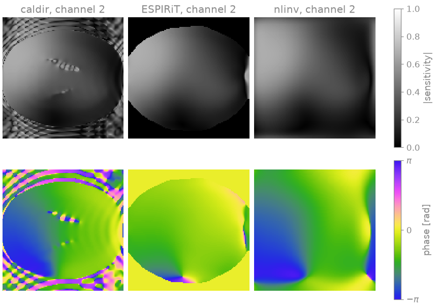
The figure shows the three estimates of one channel, magnitude above and phase below. The phase of a sensitivity map is determined only up to a phase common to all channels, which each estimator fixes differently; that common phase passes into the phase of the reconstructed image and leaves its magnitude unchanged. Up to it, the three estimates agree inside the object. They differ outside it, where the data do not determine a sensitivity: caldir divides noise by noise there and returns an arbitrary unit-modulus value, ESPIRiT sets the maps to zero, and nlinv extrapolates the smooth function its regularization favours.

Each set of sensitivities is given to bartorch.apps.pics() with the same Tikhonov weight and number of conjugate-gradient iterations, so that the reconstructions differ only in the sensitivities. The image nlinv returns jointly with its sensitivities is a fourth estimate.

reconstructions = {
    name: apps.pics(measured, maps, l2=0.001, maxiter=40)
    for name, maps in (("caldir", direct), ("ESPIRiT", espirit), ("nlinv", nonlinear))
}

for name, estimate in reconstructions.items():
    print(f"{name:>12}  NRMSE {error(estimate):.3f}")
print(f"{'nlinv image':>12}  NRMSE {error(joint):.3f}")

     caldir  NRMSE 0.025
    ESPIRiT  NRMSE 0.015
      nlinv  NRMSE 0.012
nlinv image  NRMSE 0.011

• 
• 

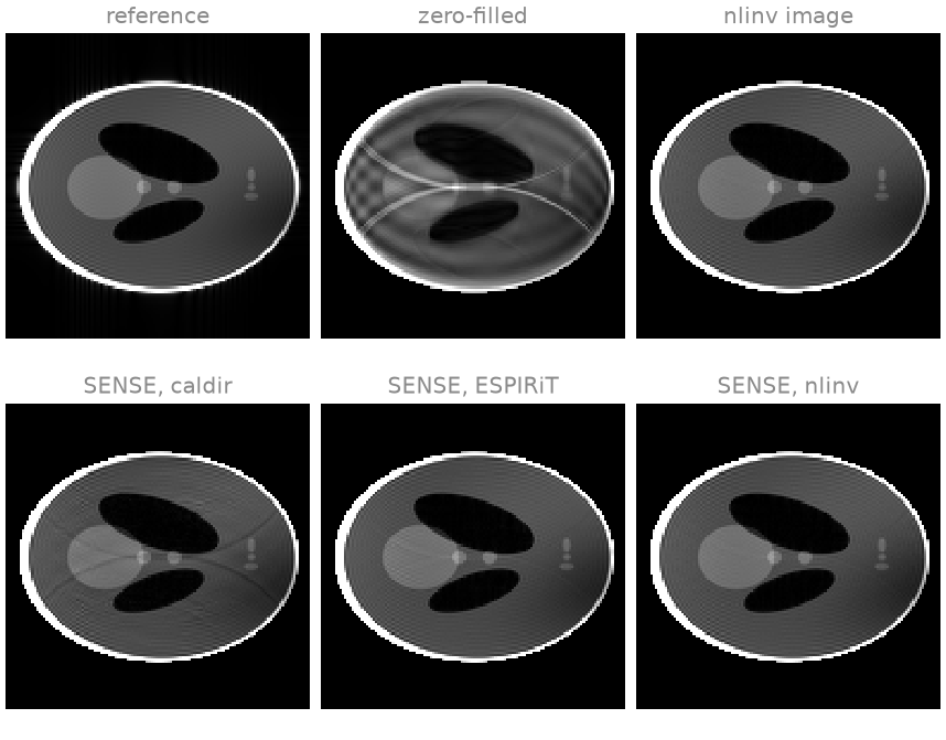
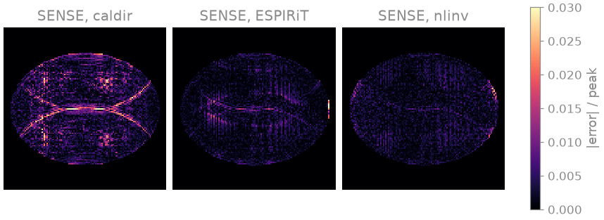
The images are windowed at half the intensity of the skull, which saturates. The zero-filled image shows the three overlapping copies of the phantom that regular undersampling produces. All three calibrations unfold them, and so does the image nlinv returns with its sensitivities. The error maps, at 3 % of the image peak, show the remaining differences: the direct estimate leaves a faint residual fold at the edges of the phantom, where its low-resolution sensitivities are least accurate, and ESPIRiT and nonlinear inversion leave mostly noise.

A smaller calibration region

ESPIRiT builds its calibration matrix from every position of a kernel, six samples wide by default, inside the ACS region. Eight lines leave three kernel positions along the phase-encoding axis, and from this data ecalib returns sensitivities that are zero in every voxel, which no reconstruction can use. caldir still runs, on an image of eight lines’ resolution. nlinv uses every acquired sample, so the calibration region affects it only through the first Gauss-Newton steps.

scarce = acquire(8)

espirit = bt.ecalib(scarce, maps=1, calib_size=8, crop=0.8)
print(f"ESPIRiT: {float((espirit.abs() > 0).float().mean()):.0%} of voxels with a sensitivity")

direct = bt.caldir(scarce, 8)
joint, estimated = bt.nlinv(scarce, maxiter=12, return_sensitivities=True)
nonlinear = estimated / bartorch.rss(estimated, axes=(0,), keepdim=True).abs().clamp(min=1e-6)

scarce_reconstructions = {
    "caldir": apps.pics(scarce, direct, l2=0.001, maxiter=40),
    "nlinv": apps.pics(scarce, nonlinear, l2=0.001, maxiter=40),
    "nlinv image": joint,
}
for name, estimate in scarce_reconstructions.items():
    print(f"{name:>12}  NRMSE {error(estimate):.3f}")

ESPIRiT: 0% of voxels with a sensitivity
      caldir  NRMSE 0.173
       nlinv  NRMSE 0.040
 nlinv image  NRMSE 0.034

• 
• 

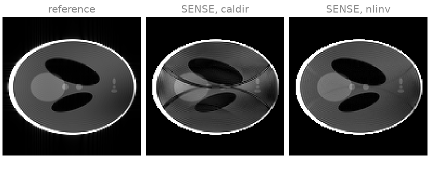
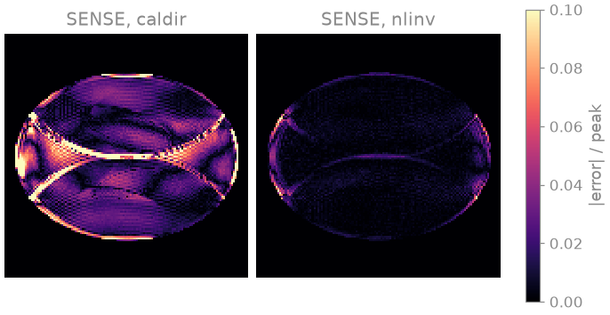
With eight ACS lines the direct estimate leaves visible residual aliasing: sensitivities estimated at a resolution of eight lines do not represent the coil profiles closely enough to unfold three copies, and the fold-over edges of the skull reappear inside the phantom. The sensitivities from nonlinear inversion still unfold the image, because they are fitted to all acquired samples. The same estimator applies to non-Cartesian data, where no Cartesian ACS region exists, as bartorch.tools.ncalib(), which Radial SENSE reconstruction uses.

The errors above are for one phantom, one noise level and one sampling pattern, and they depend on the regularization of each reconstruction; they do not rank the estimators in general.

References

[1]

Pruessmann KP, Weiger M, Scheidegger MB, Boesiger P. SENSE: sensitivity encoding for fast MRI. Magn Reson Med 42(5):952-962 (1999). https://doi.org/10.1002/(SICI)1522-2594(199911)42:5%3C952::AID-MRM16%3E3.0.CO;2-S

[2]

Uecker M, Lai P, Murphy MJ, Virtue P, Elad M, Pauly JM, Vasanawala SS, Lustig M. ESPIRiT – an eigenvalue approach to autocalibrating parallel MRI: where SENSE meets GRAPPA. Magn Reson Med 71(3):990-1001 (2014). https://doi.org/10.1002/mrm.24751

[3]

Uecker M, Hohage T, Block KT, Frahm J. Image reconstruction by regularized nonlinear inversion – joint estimation of coil sensitivities and image content. Magn Reson Med 60(3):674-682 (2008). https://doi.org/10.1002/mrm.21691