From k-space to image

This lesson reconstructs an undersampled Cartesian brain acquisition from its multichannel k-space to a coil-combined image, and shows what each step of a parallel-imaging and compressed-sensing pipeline contributes. Scan time in Cartesian MRI is proportional to the number of phase-encoding lines; skipping lines shortens the scan by the acceleration factor \(R\), but violates the Nyquist criterion and folds the image onto itself. Recovering an unaliased image from such data is what the receive coil array, and prior knowledge of the image, are used for.

The acquisition is simulated from a BrainWeb tissue segmentation and the eight channels of BART’s head-coil model, with one line in three acquired along the phase-encoding direction. The pipeline consists of coil compression, sensitivity calibration by ESPIRiT, and a regularized least-squares fit of the SENSE forward model

\[y = P F S x + \varepsilon,\]

with \(S\) the coil sensitivities, \(F\) the Fourier transform, \(P\) the sampling operator that keeps the acquired phase encodes, and \(\varepsilon\) complex Gaussian noise. The MRI encoding operator states the model and Inverse problems and their solvers the estimator.

Shapes are C order, so a Cartesian k-space is (coils, z, y, x) with the readout along x and the phase encoding along y; see Data layout and conventions.

Learning objectives

• Simulate a multichannel Cartesian acquisition from a tissue segmentation.

• Undersample the phase-encoding direction with a variable-density pattern around a fully sampled autocalibration (ACS) region.

• Compress the channels with bartorch.tools.cc() and estimate their sensitivities with bartorch.tools.ecalib().

• Reconstruct with bartorch.apps.pics(), with a Tikhonov and with a wavelet sparsity penalty, and compare the results by error maps, NRMSE and SSIM.

It builds on the conventions of Tensors and commands. The sections after it examine calibration, regularization and the operator form of each step in turn; the next lesson, Coil sensitivity calibration, compares sensitivity estimators.

import csv
from pathlib import Path

import brainweb_dl
import numpy as np
import torch
from brainweb_dl import get_mri

import bartorch
import bartorch.tools as bt
from bartorch import apps, priors

Phantom

BrainWeb [1] publishes a segmentation rather than an image: one membership map per tissue class, from which a table of relaxation times and proton densities gives the signal of a chosen acquisition. The volume brainweb-dl returns is indexed (inferior-superior, posterior-anterior, left-right), so its first axis selects an axial slice, and an image is drawn from its first row down, so flipping it puts anterior at the top.

SIZE = 192
COILS = 8
SLICE = 90  # axial, through the lateral ventricles
TISSUES = (1, 2, 3, 4, 5, 6, 8)  # everything the table gives relaxation times

table = Path(brainweb_dl.__file__).parent / "data" / "brainweb1_tissues.csv"
entries = list(csv.DictReader(table.open()))
tissue_t1 = np.array([float(row["T1 (ms)"]) for row in entries], dtype=np.float32)[list(TISSUES)]
tissue_t2 = np.array([float(row["T2 (ms)"]) for row in entries], dtype=np.float32)[list(TISSUES)]
tissue_pd = np.array([float(row["PD (ms)"]) for row in entries], dtype=np.float32)[list(TISSUES)]

fractions = np.flipud(get_mri(sub_id=0, contrast="fuzzy")[SLICE])[..., list(TISSUES)].copy()

The slice is cropped to a square field of view around the head and resampled to the matrix reconstructed here. The crop leaves a margin, as a real field of view does: the aliased copies of an undersampled acquisition then fall partly outside the head.

MARGIN = 0.25

A membership-weighted average of the table gives \(T_1\), \(T_2\) and the proton density at every voxel, and the spin-echo signal

\[S = \rho \, \left(1 - e^{-T_R/T_1}\right) e^{-T_E/T_2}\]

turns those into the image the experiment measures. At a short repetition time and a short echo time the contrast is \(T_1\)-weighted: white matter bright, cerebrospinal fluid dark, subcutaneous fat brightest of all.

TR, TE = 600.0, 12.0  # ms

weights = memberships * torch.as_tensor(tissue_pd)[:, None, None]
share = weights.sum(0).clamp(min=1e-6)
T1 = (weights * torch.as_tensor(tissue_t1)[:, None, None]).sum(0) / share
T2 = (weights * torch.as_tensor(tissue_t2)[:, None, None]).sum(0) / share
proton_density = weights.sum(0) / weights.sum(0).max()

signal = (
    proton_density * (1 - torch.exp(-TR / T1.clamp(min=1e-3))) * torch.exp(-TE / T2.clamp(min=1e-3))
)
signal = torch.where(T1 > 0, signal, torch.zeros(()))
signal = signal / signal.max()

# A smooth quadratic phase stands in for the transmit and off-resonance phase
# of a real object, so that nothing below depends on the image being real.
grid_y, grid_x = torch.meshgrid(
    torch.linspace(-1.0, 1.0, SIZE), torch.linspace(-1.0, 1.0, SIZE), indexing="ij"
)
image = (signal * torch.exp(0.8j * (grid_x**2 - 0.5 * grid_y**2))).to(torch.complex64)

Coils

Each receive channel measures the object weighted by its complex sensitivity profile, \(x_c = S_c x\). The sensitivities here are BART’s analytical head coil, evaluated on the image grid that bartorch.tools.grid() describes. Dividing them by their root sum of squares over the channels normalizes \(\sum_c |S_c|^2\) to one, so that the optimal coil combination of the coil images is the image itself and a reconstruction can be compared against it directly. Complex Gaussian noise is then added to every k-space sample, as thermal noise is in the receiver chain.

sensitivities = bt.coils(t=bt.grid(D=(SIZE, SIZE, 1)), n=COILS)[:, 0]
sensitivities = sensitivities / bartorch.rss(sensitivities, axes=(0,), keepdim=True)

coil_images = sensitivities * image
kspace = bartorch.fft(coil_images, axes=(-2, -1), unitary=True)
kspace = bt.noise(kspace, n=1e-4, s=42)

• 
• 

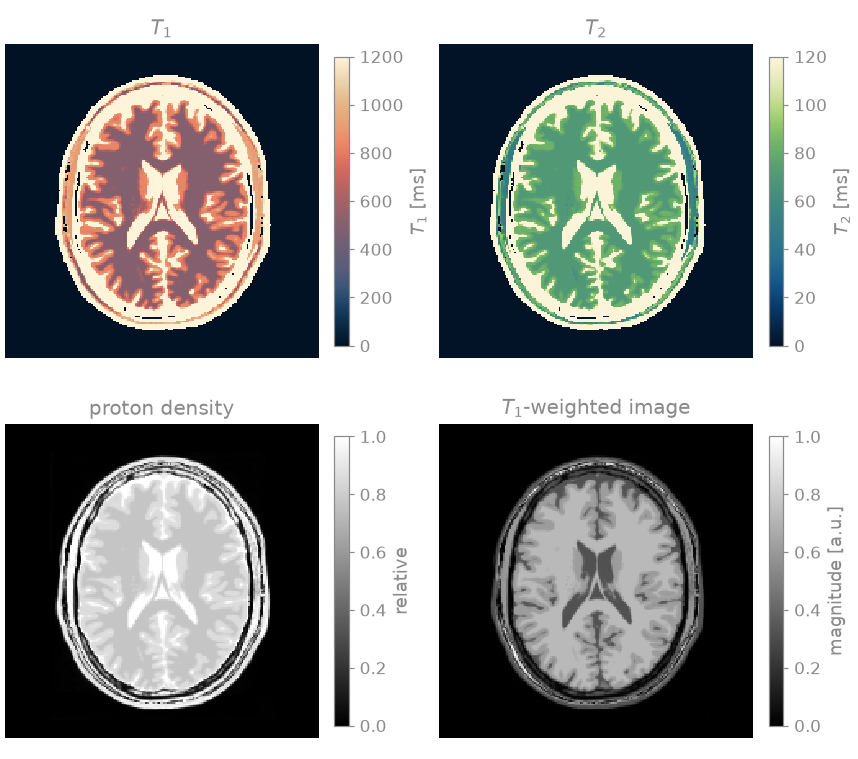
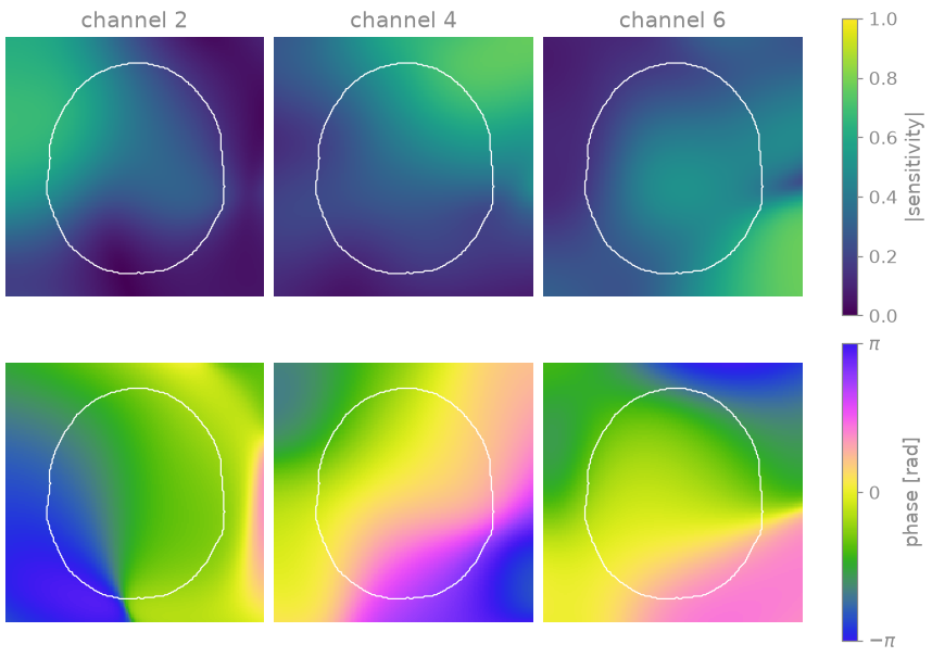
The first figure is the ground truth: the relaxation maps, drawn with the perceptually uniform colormaps recommended for relaxometry [2] – lipari for \(T_1\), navia for \(T_2\) – and with a window that stops short of cerebrospinal fluid, the proton density, and the \(T_1\)-weighted image they give. The second shows three of the eight sensitivities, magnitude above and phase below, with the outline of the head. Each magnitude is highest near its coil element and falls off across the head; the phase varies smoothly. These spatial variations are the extra encoding that parallel imaging uses to separate aliased voxels.

Sampling

The readout is fully sampled, since it costs no scan time, and a subset of the phase encodes is acquired. The lines are drawn at random from a variable density that is highest at the k-space centre, where most of the signal energy is, with a block of 24 central lines, the autocalibration signal (ACS) region, acquired in full. ESPIRiT reads its calibration matrix from the ACS region, so an acquisition without one would need a separate calibration scan. The pattern is a column vector along the phase-encoding direction: it broadcasts over the readout and over the channels.

ACCELERATION = 3
CALIBRATION = 24

encodes = torch.arange(SIZE) - SIZE // 2
profile = (1.0 + 2.0 * encodes.abs() / SIZE) ** -3.0
centre = (encodes.abs() < CALIBRATION // 2).to(torch.float32)
drawn = torch.multinomial(
    profile * (1.0 - centre),
    SIZE // ACCELERATION - CALIBRATION,
    replacement=False,
    generator=torch.Generator().manual_seed(11),
)
lines = centre.clone()
lines[drawn] = 1.0

pattern = lines.reshape(SIZE, 1).to(torch.complex64)
measured = kspace[:, None] * pattern

print(f"{int(lines.sum())} of {SIZE} phase encodes acquired, R = {SIZE / lines.sum():.1f}")

63 of 192 phase encodes acquired, R = 3.0

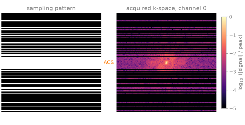
In the pattern (readout horizontal, phase encoding vertical) every acquired phase encode is a full line; the lines cluster towards the centre and the ACS band is dense.

Channel compression

Eight channels carry less independent information than eight images: the sensitivities overlap, and the singular value spectrum of the calibration matrix falls off. bartorch.tools.cc() returns the matrix that projects the channels onto their leading singular vectors [3], the virtual coils, and bartorch.tools.ccapply() applies it. Calibration, the encoding operator and every iteration then cost six channels rather than eight, at a negligible loss of the encoding capacity of the array.

VIRTUAL = 6

matrix = bt.cc(measured, p=VIRTUAL, M=True, r=CALIBRATION)
compressed = bt.ccapply(measured, matrix, p=VIRTUAL)

Sensitivity calibration

ESPIRiT [4] estimates the sensitivities from the ACS region alone: it builds a calibration matrix from all k-space neighbourhoods (kernels) in the region, and obtains the sensitivities at each voxel as the eigenvector of an operator derived from that matrix whose eigenvalue is one. Outside the object no eigenvalue is close to one; crop sets the maps to zero where the eigenvalue falls below it, which keeps the background out of the reconstruction.

maps = bt.ecalib(compressed, maps=1, calib_size=CALIBRATION, crop=0.8)

Reconstruction

Three reconstructions of the same data are compared.

• The zero-filled reconstruction sets the missing phase encodes to zero, inverse-transforms each channel and combines them by root sum of squares. It uses no model of the encoding, so every missing line leaves aliasing.

• SENSE [5] solves \(\min_x \|PFSx - y\|_2^2 + \lambda\|x\|_2^2\) by conjugate gradients. The sensitivities unfold the aliasing, but the inversion amplifies the noise by the g-factor, which is highest where the coils cannot distinguish aliased voxels.

• Compressed sensing [6] replaces the Tikhonov term by an \(\ell_1\) penalty on the wavelet coefficients, solved by FISTA [7]. The random undersampling makes the aliasing incoherent, i.e. noise-like in the wavelet domain, and the sparsity penalty removes it together with the amplified noise.

channel_images = bartorch.ifft(compressed[:, 0], axes=(-2, -1), unitary=True)
zero_filled = bartorch.rss(channel_images, axes=(0,))

sense = apps.pics(compressed, maps, l2=0.001, maxiter=60)
wavelet = apps.pics(
    compressed,
    maps,
    regularizers=priors.Wavelet((-1, -2), 0.004),
    solver="fista",
    maxiter=100,
)

The sensitivities ESPIRiT estimates and the ones the acquisition was simulated with differ by a phase that varies from voxel to voxel, so the reconstructed image does too, and the comparison is between magnitudes. pics returns the image in the units of the data it scaled, so bartorch.tools.nrmse() is called with scaled=True, which fits a global factor before comparing.

results = {"zero-filled": zero_filled, "SENSE": sense, "wavelet CS": wavelet}
for name, estimate in results.items():
    error = bt.nrmse(image.abs(), estimate.abs(), scaled=True)
    similarity = bt.ssim(image.abs(), scaled(estimate, image))
    print(f"{name:>12}  NRMSE {error:.3f}  SSIM {similarity:.3f}")

zero-filled  NRMSE 0.129  SSIM 0.541
      SENSE  NRMSE 0.101  SSIM 0.737
 wavelet CS  NRMSE 0.044  SSIM 0.926

• 
• 
• 

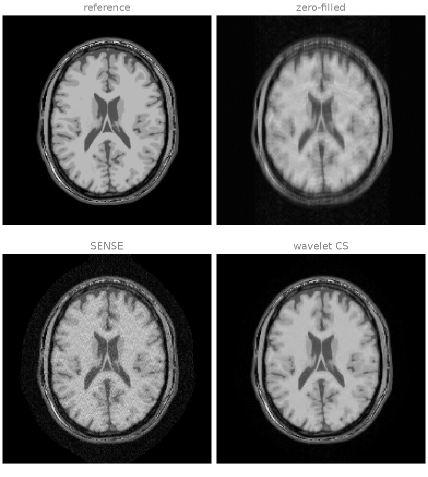
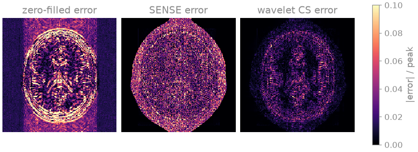
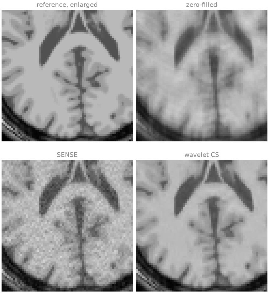
The zero-filled image carries the aliasing of the missing phase encodes as blurring and ghosting along the vertical, phase-encoding direction. SENSE removes the coherent aliasing, but its error map shows noise amplified in the centre of the head, where the coil sensitivities are least distinct, and incoherent residual artefacts of the random sampling. The wavelet penalty suppresses both; in the enlarged region the cortical folding and the ventricle boundaries are sharper and the background of the brain is smooth. The NRMSE and SSIM printed above quantify the same ordering.

How much the penalty removes depends on its weight, which is chosen here and not estimated: a larger weight removes more noise and more fine texture with it. Coil sensitivity calibration compares sensitivity estimators, and Regularized reconstruction varies the weight.

References

[1]

Collins DL, Zijdenbos AP, Kollokian V, Sled JG, Kabani NJ, Holmes CJ, Evans AC. Design and construction of a realistic digital brain phantom. IEEE Trans Med Imaging 17(3):463-468 (1998). https://doi.org/10.1109/42.712135

[2]

Fuderer M, Wichtmann B, Crameri F, de Souza NM, Baeßler B, Gulani V, et al. Color-map recommendation for MR relaxometry maps. Magn Reson Med 93(2):490-506 (2025). https://doi.org/10.1002/mrm.30290

[3]

Huang F, Vijayakumar S, Li Y, Hertel S, Duensing GR. A software channel compression technique for faster reconstruction with many channels. Magn Reson Imaging 26(1):133-141 (2008). https://doi.org/10.1016/j.mri.2007.04.010

[4]

Uecker M, Lai P, Murphy MJ, Virtue P, Elad M, Pauly JM, Vasanawala SS, Lustig M. ESPIRiT – an eigenvalue approach to autocalibrating parallel MRI: where SENSE meets GRAPPA. Magn Reson Med 71(3):990-1001 (2014). https://doi.org/10.1002/mrm.24751

[5]

Pruessmann KP, Weiger M, Scheidegger MB, Boesiger P. SENSE: sensitivity encoding for fast MRI. Magn Reson Med 42(5):952-962 (1999). https://doi.org/10.1002/(SICI)1522-2594(199911)42:5%3C952::AID-MRM16%3E3.0.CO;2-S

[6]

Lustig M, Donoho D, Pauly JM. Sparse MRI: the application of compressed sensing for rapid MR imaging. Magn Reson Med 58(6):1182-1195 (2007). https://doi.org/10.1002/mrm.21391

[7]

Beck A, Teboulle M. A fast iterative shrinkage-thresholding algorithm for linear inverse problems. SIAM J Imaging Sci 2(1):183-202 (2009). https://doi.org/10.1137/080716542