Noise prewhitening

This lesson measures how correlated noise between receive channels lowers the signal-to-noise ratio (SNR) of a SENSE reconstruction, and how much of it prewhitening with a noise-only acquisition recovers.

The thermal noise of a receive array is correlated between channels, through mutual inductance between the coil elements and shared noise sources in the sample, and its level differs from one channel to another, through the elements’ size, loading and preamplifier gain. Least squares is the maximum-likelihood estimator only for white noise, i.e. for a channel noise covariance proportional to the identity. A reconstruction that ignores the covariance \(\Psi\) weights every channel equally and does not combine them with the optimal SNR [1]. Prewhitening transforms the data by a matrix \(W\) with \(W \Psi W^H = I\), which makes the channel noise white; the sensitivities are then calibrated on, and the SENSE reconstruction run on, the whitened channels unchanged [2]. \(\Psi\) is estimated from a noise scan, an acquisition with the RF transmitter off that most vendors run before every protocol.

The SNR of the two reconstructions is measured by the pseudo-replica method [3]: the same reconstruction is repeated on independent noise realizations added to one noise-free acquisition, and the standard deviation across repetitions is the noise of each voxel. This is how SNR and g-factor maps are obtained for iterative reconstructions, for which no closed-form noise propagation exists.

The phantom and the coil sensitivities are built as in From k-space to image; the cell that does it is hidden on this page and present in the script this page can be downloaded as.

Learning objectives

• Estimate the channel noise covariance from a noise scan and whiten the data with bartorch.tools.whiten().

• Measure an SNR map by the pseudo-replica method.

• Quantify the SNR gain that prewhitening gives a SENSE reconstruction.

It follows Nonlinear inversion. The next section starts with Regularized reconstruction.

import csv
from pathlib import Path

import brainweb_dl
import numpy as np
import torch
from brainweb_dl import get_mri

import bartorch
import bartorch.tools as bt
from bartorch import apps

SIZE = 128
COILS = 8

Correlated channel noise

The noise covariance of the simulation couples the channels by a correlation coefficient falling as \(0.5^{|i-j|}\) with the distance between their indices, and gives the channels noise standard deviations between 0.6 and 1.6 times a common level. The noise scan measures the same channels without signal; its sample covariance is the estimate of \(\Psi\) that bartorch.tools.whiten() inverts.

SIGMA = 0.01  # noise level, relative to the image's peak

channels = torch.arange(COILS)
levels = torch.linspace(0.6, 1.6, COILS)
correlation = 0.5 ** (channels[:, None] - channels[None, :]).abs().float()
covariance = levels[:, None] * correlation * levels[None, :]
mixing = torch.linalg.cholesky(covariance).to(torch.complex64)
generator = torch.Generator().manual_seed(2)


def channel_noise(shape):
    """Complex Gaussian noise with the channel covariance above."""
    white = torch.randn(COILS, *shape, generator=generator)
    white = (white + 1j * torch.randn(COILS, *shape, generator=generator)) / 2**0.5
    return SIGMA * torch.einsum("ij,j...->i...", mixing, white.to(torch.complex64))


noise_scan = channel_noise((SIZE, SIZE))[:, None]

The whitening matrix maps the measured covariance to the identity. The measure printed below is the mean magnitude of the off-diagonal covariance entries relative to the mean diagonal entry, which is zero for uncorrelated channels.

def channel_covariance(samples):
    """Sample covariance of the channels, over every other axis."""
    flat = samples.reshape(COILS, -1)
    return (flat @ flat.conj().T) / flat.shape[1]


def off_diagonal(matrix):
    diagonal = torch.diagonal(matrix).abs()
    return float((matrix.abs().sum() - diagonal.sum()) / (COILS * (COILS - 1)) / diagonal.mean())


measured = channel_covariance(noise_scan)
whitened = channel_covariance(bt.whiten(noise_scan, noise_scan))

print(f"off-diagonal covariance: {off_diagonal(measured):.3f} measured")
print(f"                         {off_diagonal(whitened):.3f} after whitening")

off-diagonal covariance: 0.202 measured
                         0.000 after whitening

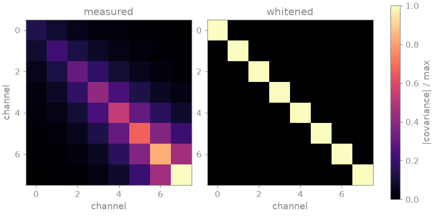
The measured covariance has a strong diagonal whose entries grow with the channel index, the unequal noise levels, and off-diagonal bands, the correlation. After whitening it is the identity.

Acquisition and calibration

Every second phase encode is acquired (\(R = 2\)), with 24 central lines kept as the ACS region. Each pseudo-replica adds a new noise realization to the same noise-free k-space. The sensitivities are calibrated once per pipeline, from the first replica: from the channels as measured, and from the whitened channels.

CALIBRATION = 24
REPLICAS = 32

lines = torch.zeros(SIZE)
lines[::2] = 1.0
lines[SIZE // 2 - CALIBRATION // 2 : SIZE // 2 + CALIBRATION // 2] = 1.0
pattern = lines.reshape(SIZE, 1).to(torch.complex64)

noiseless = bartorch.fft(sensitivities * image, axes=(-2, -1), unitary=True)


def acquire():
    """One replica: the noise-free k-space plus new noise, sampled."""
    return ((noiseless + channel_noise((SIZE, SIZE))) * pattern)[:, None]


first = acquire()
maps_measured = bt.ecalib(first, maps=1, calib_size=CALIBRATION, crop=0.8)
maps_whitened = bt.ecalib(bt.whiten(first, noise_scan), maps=1, calib_size=CALIBRATION, crop=0.8)

Pseudo-replicas

Both pipelines use the same reconstruction, conjugate-gradient SENSE with a small Tikhonov weight and a fixed number of iterations; they differ only in whether the data are whitened first.

plain, prewhitened = [], []
for _ in range(REPLICAS):
    data = acquire()
    plain.append(apps.pics(data, maps_measured, l2=1e-3, maxiter=30))
    prewhitened.append(apps.pics(bt.whiten(data, noise_scan), maps_whitened, l2=1e-3, maxiter=30))

plain, prewhitened = torch.stack(plain), torch.stack(prewhitened)

The SNR of a voxel is the magnitude of the mean reconstruction over the standard deviation across replicas. Both are reported over the white matter, where the phantom is homogeneous.

white_matter = memberships[CLASS["WM"]] > 0.8


def snr_map(replicas):
    return replicas.mean(0).abs() / replicas.std(0)


for name, replicas in (("as measured", plain), ("prewhitened", prewhitened)):
    values = snr_map(replicas)[white_matter]
    mean, median = float(values.mean()), float(values.median())
    print(f"{name:>12}  white-matter SNR {mean:6.1f} (median {median:.1f})")

gain = snr_map(prewhitened) / snr_map(plain)
print(f"SNR ratio, prewhitened over as measured: {float(gain[white_matter].median()):.2f} (median)")

 as measured  white-matter SNR   38.1 (median 37.7)
 prewhitened  white-matter SNR   55.6 (median 54.3)
SNR ratio, prewhitened over as measured: 1.42 (median)

• 
• 

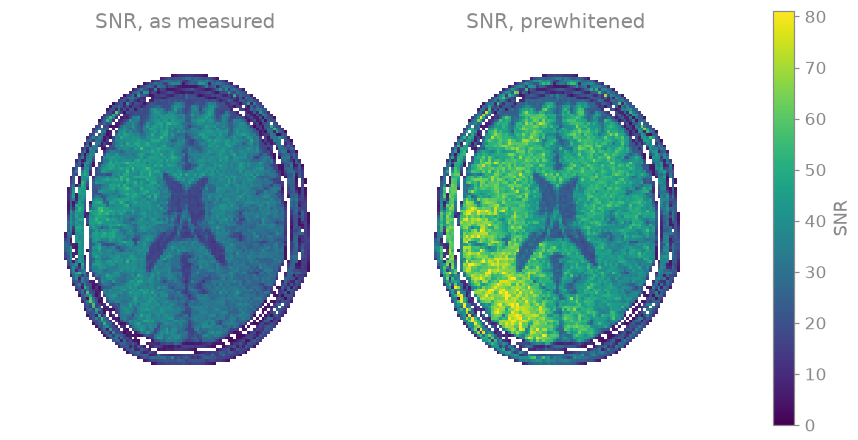
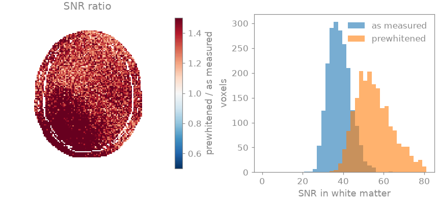
Prewhitening raises the SNR throughout the head, and the white-matter histogram shifts by the ratio printed above. The gain varies in space: it is largest in the posterior half of the head, where the channels with the lowest noise level (the first channels here) are most sensitive. Without whitening the least-squares fit weights those channels no more than the noisiest ones; after whitening each channel enters with the weight its noise level warrants. The size of the gain depends on the array’s noise correlation and on the spread of its channel noise levels, and is measured here for one simulated covariance; with uncorrelated channels of equal noise level it is one.

References

[1]

Roemer PB, Edelstein WA, Hayes CE, Souza SP, Mueller OM. The NMR phased array. Magn Reson Med 16(2):192-225 (1990). https://doi.org/10.1002/mrm.1910160203

[2]

Pruessmann KP, Weiger M, Börnert P, Boesiger P. Advances in sensitivity encoding with arbitrary k-space trajectories. Magn Reson Med 46(4):638-651 (2001). https://doi.org/10.1002/mrm.1241

[3]

Robson PM, Grant AK, Madhuranthakam AJ, Lattanzi R, Sodickson DK, McKenzie CA. Comprehensive quantification of signal-to-noise ratio and g-factor for image-based and k-space-based parallel imaging reconstructions. Magn Reson Med 60(4):895-907 (2008). https://doi.org/10.1002/mrm.21728