Trajectories and transforms

This lesson introduces the building blocks of non-Cartesian reconstruction: radial, golden-angle and spiral trajectories, the non-uniform fast Fourier transform (NUFFT) that samples an image along them, the density compensation that an adjoint (gridding) reconstruction needs, and the point spread function (PSF) that describes the undersampling artefacts.

Non-Cartesian trajectories sample k-space along curves rather than on a grid. Radial and spiral readouts start at the k-space centre, which makes them robust to motion and flow and lets them oversample the low spatial frequencies; they are the basis of real-time, ultrashort-echo-time and free-breathing imaging. Their samples do not lie on the Cartesian grid, so the FFT is replaced by the NUFFT. Every non-Cartesian transform in bartorch is computed by FINUFFT [1], which evaluates

\[y_j = \frac{1}{\sqrt{N}} \sum_{m} x_m \, \exp\!\Big(-2\pi i \sum_d \frac{k_{j,d}\, m_d}{n_d}\Big)\]

to a requested tolerance, with the sum over the \(N\) voxels \(m\) of an image of \(n_d\) voxels along dimension \(d\), and \(k_j\) in grid units. The spreading kernel and the deapodization are FINUFFT’s, sized from the tolerance: Non-Cartesian sampling states the conventions and the accuracy.

The phantom is built as in From k-space to image; the cell that does it is hidden on this page and present in the script this page can be downloaded as.

Learning objectives

• Generate radial and golden-angle trajectories in grid units with bartorch.tools.traj(), and a spiral trajectory directly.

• Apply bartorch.nufft() and bartorch.nufft_adjoint(), and check the transform against the sum that defines it.

• Explain why a gridding reconstruction needs density compensation, and compute the weights analytically and with bartorch.estimate_density().

• Compare the normal operator as a convolution with the transform pair, and relate the PSF of an undersampled radial trajectory to its streak artefacts.

It follows Operators and solvers. The next lesson, Radial SENSE reconstruction, reconstructs an undersampled radial acquisition.

import csv
import time
from pathlib import Path

import brainweb_dl
import numpy as np
import torch
from brainweb_dl import get_mri

import bartorch
import bartorch.tools as bt
from bartorch import linop

SIZE = 128

Trajectories

A trajectory is (*encoding, shots, samples, 3) in grid units: the coordinates of every sample, in units of the k-space cell of the image it encodes, so a readout of SIZE samples runs from \(-n/2\) to \(n/2\) for an image of \(n\) voxels along the readout. The third component is \(k_z\), zero throughout for a two-dimensional trajectory, and whether it is used determines whether the transform is two- or three-dimensional.

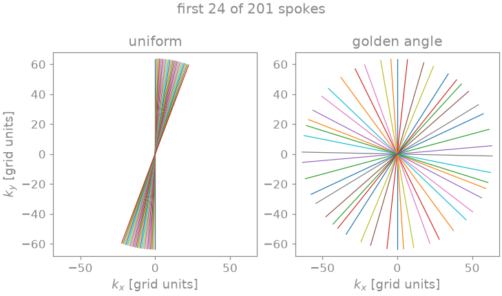
Successive spokes are separated either by \(\pi\) over their number, which tiles k-space uniformly for one frame, or by the golden angle, which tiles it approximately uniformly for any number of consecutive spokes [2]. Only the second lets an acquisition be cut into frames after it was measured, as Dynamic golden-angle radial MRI does.

SPOKES = 201  # pi/2 * SIZE, the number at which radial sampling is not undersampled

uniform = bt.traj(readout=SIZE, spokes=SPOKES, radial=True)
golden = bt.traj(readout=SIZE, spokes=SPOKES, radial=True, golden=True)

print(f"{tuple(golden.shape)}: {SPOKES} shots of {SIZE} samples")

(201, 128, 3): 201 shots of 128 samples

The transform

bartorch.nufft() samples an image along a trajectory and bartorch.nufft_adjoint() maps samples back onto a grid. The samples an acquisition would measure are the transform of the image; below they are checked against the sum that defines them, evaluated in double precision over one spoke, which is a reference outside BART and outside FINUFFT.

samples = bartorch.nufft(image, golden)
print(f"samples {tuple(samples.shape)}")

spoke = golden[0].real.to(torch.float64)
axis_y, axis_x = torch.meshgrid(
    torch.arange(SIZE) - SIZE // 2, torch.arange(SIZE) - SIZE // 2, indexing="ij"
)
phase = (
    -2j
    * np.pi
    / SIZE
    * (
        spoke[:, 0:1] * axis_x.reshape(1, -1).to(torch.float64)
        + spoke[:, 1:2] * axis_y.reshape(1, -1).to(torch.float64)
    )
)
explicit = torch.exp(phase) @ image.to(torch.complex128).reshape(-1, 1) / SIZE

difference = float((explicit - samples[0]).abs().max() / explicit.abs().max())
print(f"largest relative difference from the explicit sum: {difference:.1e}")

samples (201, 128, 1)
largest relative difference from the explicit sum: 1.9e-04

The transform is planned to a tolerance rather than computed exactly, and the difference above is within the tolerance it was planned with: a thousandth by default, on a grid a quarter larger than the image. The default is chosen for reconstruction, where the transform’s error is intended to stay small beside the effect of noise and undersampling; bartorch.linop.NUFFT takes oversampling and width where more accuracy is needed.

Density compensation

The adjoint is not the inverse. Every spoke passes through the centre of k-space, so the radial sampling density falls as \(1/\lvert k \rvert\) and the adjoint overweights low frequencies. The weight that compensates for it is the inverse sampling density [3], which for radial sampling is proportional to the distance from the centre.

radius = torch.linalg.norm(golden.real[..., :2], dim=-1, keepdim=True)
weights = radius.clamp(min=0.25).to(torch.complex64)

plain = bartorch.nufft_adjoint(samples, golden, image_shape=(SIZE, SIZE))
compensated = bartorch.nufft_adjoint(samples * weights, golden, image_shape=(SIZE, SIZE))

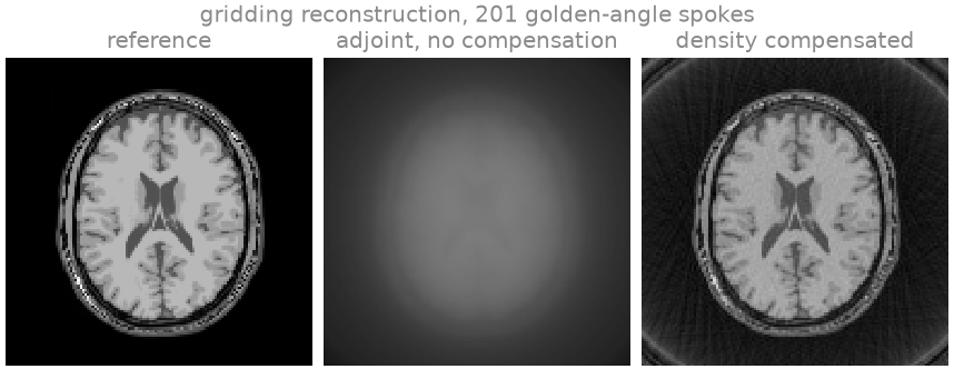
The uncompensated adjoint is the image convolved with the point spread function, the inverse Fourier transform of the sampling density; the density is concentrated at the centre of k-space, so the result is blurred. The compensated adjoint resolves the tissue boundaries. Neither recovers the k-space the trajectory does not reach: a radial acquisition samples a disc, so the frequencies in the corners of the Cartesian grid are missing whatever the weights are.

Estimated density

The ramp \(\lvert k \rvert\) is the density of an ideal radial trajectory. bartorch.estimate_density() estimates the density of any trajectory by the fixed-point iteration of Pipe and Menon [3], evaluated with the same non-uniform transforms, and returns weights for each sample. It takes the coordinates as (..., samples, 2), so the spokes are flattened into one list of samples.

estimated = bartorch.estimate_density(golden.real[..., :2].reshape(-1, 2), (SIZE, SIZE))
estimated = estimated.reshape(SPOKES, SIZE, 1).to(torch.complex64)

for name, density in (("ramp", weights), ("Pipe-Menon", estimated)):
    adjoint = bartorch.nufft_adjoint(samples * density, golden, image_shape=(SIZE, SIZE))
    print(f"{name:>10}  NRMSE {bt.nrmse(image.abs(), adjoint.abs(), scaled=True):.3f}")

      ramp  NRMSE 0.297
Pipe-Menon  NRMSE 0.278

For a radial trajectory the two weightings give similar errors, both of which include the k-space corners the disc does not cover. The estimate matters where no closed form is at hand. A spiral interleaf is not generated by bartorch.tools.traj(), and is written here as an Archimedean spiral: sixteen interleaves reaching \(\pm n/2\), with \(n / 32\) turns each so that adjacent turns are one grid unit apart, the radial Nyquist spacing, and 1024 samples per interleaf.

INTERLEAVES, READOUT = 16, 1024

progress = torch.linspace(0.0, 1.0, READOUT)
radius = SIZE / 2 * progress
angle = 2 * np.pi * SIZE / (2 * INTERLEAVES) * progress
spiral = torch.stack(
    [
        torch.stack(
            [
                radius * torch.cos(angle + 2 * np.pi * arm / INTERLEAVES),
                radius * torch.sin(angle + 2 * np.pi * arm / INTERLEAVES),
                torch.zeros(READOUT),
            ],
            dim=-1,
        )
        for arm in range(INTERLEAVES)
    ]
)

spiral_samples = bartorch.nufft(image, spiral)
spiral_density = bartorch.estimate_density(spiral[..., :2].reshape(-1, 2), (SIZE, SIZE))
spiral_density = spiral_density.reshape(INTERLEAVES, READOUT, 1).to(torch.complex64)

spiral_plain = bartorch.nufft_adjoint(spiral_samples, spiral, image_shape=(SIZE, SIZE))
spiral_compensated = bartorch.nufft_adjoint(
    spiral_samples * spiral_density, spiral, image_shape=(SIZE, SIZE)
)
for name, adjoint in (("adjoint", spiral_plain), ("compensated", spiral_compensated)):
    print(f"spiral {name:>12}  NRMSE {bt.nrmse(image.abs(), adjoint.abs(), scaled=True):.3f}")

spiral      adjoint  NRMSE 0.693
spiral  compensated  NRMSE 0.089

• 
• 

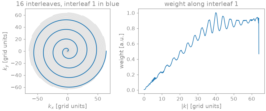
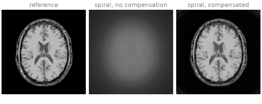
The estimated weight of an Archimedean spiral grows with the radius: the interleaves are separated by a constant distance while the arc length traversed per sample grows, so the samples are densest at the centre. The weight oscillates with the period of the turns, levels off in the outer part of k-space, and drops over the last samples, where the outermost turn has no neighbour outside it. Without compensation the spiral adjoint is dominated by the densely sampled low spatial frequencies and appears as a blurred, low-contrast image; with the estimated weights the tissue contrast and the edges are restored, which the NRMSE printed above quantifies.

The normal operator

bartorch.linop.NUFFT is the transform as an operator, and carries the weights and a subspace basis where there are any, because its normal operator \(A^H A\) is built over both. That normal is a convolution with a point spread function on a doubled grid rather than a transform each way [4], which is what a solver applies once per iteration.

A = linop.NUFFT(golden, image_shape=(SIZE, SIZE))

repeats = 5
start = time.perf_counter()
for _ in range(repeats):
    toeplitz = A.gram()(image)
convolution = (time.perf_counter() - start) / repeats

start = time.perf_counter()
for _ in range(repeats):
    pair = A.H(A(image))
transforms = (time.perf_counter() - start) / repeats

print(f"A^H A as a convolution   {1e3 * convolution:6.1f} ms")
print(f"A^H A as two transforms  {1e3 * transforms:6.1f} ms")
print(f"relative difference      {float((toeplitz - pair).abs().max() / pair.abs().max()):.1e}")

A^H A as a convolution      0.5 ms
A^H A as two transforms     0.8 ms
relative difference      2.7e-03

The two agree to a small multiple of the transform’s tolerance.

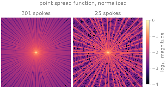
bartorch.tools.psf() computes that function on its own. Its extent is the aliasing the trajectory produces: for a fully sampled radial trajectory it is a central peak with a low, broad skirt, and undersampling raises the skirt into the streaks a radial reconstruction is known for.

fully_sampled = bt.psf(bt.traj(readout=SIZE, spokes=SPOKES, radial=True, golden=True))
undersampled = bt.psf(bt.traj(readout=SIZE, spokes=SPOKES // 8, radial=True, golden=True))

A reconstruction that uses all of this – the transform, the weights, the sensitivities and the normal operator – is Radial SENSE reconstruction.

References

[1]

Barnett AH, Magland J, af Klinteberg L. A parallel nonuniform fast Fourier transform library based on an “exponential of semicircle” kernel. SIAM J Sci Comput 41(5):C479-C504 (2019). https://doi.org/10.1137/18M120885X

[2]

Winkelmann S, Schaeffter T, Koehler T, Eggers H, Doessel O. An optimal radial profile order based on the Golden Ratio for time-resolved MRI. IEEE Trans Med Imaging 26(1):68-76 (2007). https://doi.org/10.1109/TMI.2006.885337

[3] (1,2)

Pipe JG, Menon P. Sampling density compensation in MRI: rationale and an iterative numerical solution. Magn Reson Med 41(1):179-186 (1999). https://doi.org/10.1002/(SICI)1522-2594(199901)41:1%3C179::AID-MRM25%3E3.0.CO;2-V

[4]

Fessler JA, Lee S, Olafsson VT, Shi HR, Noll DC. Toeplitz-based iterative image reconstruction for MRI with correction for magnetic field inhomogeneity. IEEE Trans Signal Process 53(9):3393-3402 (2005). https://doi.org/10.1109/TSP.2005.853152