Dynamic golden-angle radial MRI

This lesson reconstructs a dynamic contrast-enhanced series from one continuous golden-angle radial acquisition, cut into frames of thirteen spokes each. Each frame on its own is undersampled fifteenfold and cannot be reconstructed; the series can, because consecutive frames are strongly correlated, and a total-variation penalty along the time axis states that correlation. The lesson compares frame-by-frame gridding with this joint reconstruction on the images and on the time-intensity curve a perfusion analysis would use.

In a golden-angle acquisition [1] each spoke is rotated from the previous one by \(180^\circ / \phi \approx 111.25^\circ\), with \(\phi\) the golden ratio, so that any block of consecutive spokes covers k-space approximately uniformly, whatever its length and wherever it starts. The acquisition therefore runs without interruption, and the temporal resolution is chosen at reconstruction: fewer spokes per frame give a finer temporal resolution and stronger streak artefacts. Combined with parallel imaging and a sparsity penalty along time, this is GRASP [2].

The encoding is that of Radial SENSE reconstruction with a frame axis added: the image is (frames, y, x), the trajectory indexes frames as well as spokes, and the coil sensitivities are shared by all frames. The phantom and the coil sensitivities are built as in From k-space to image; the cell that does it is hidden on this page and present in the script this page can be downloaded as.

Learning objectives

• Divide a continuous golden-angle acquisition into frames after the fact.

• Build an encoding whose image and trajectory carry a frame axis.

• Regularize along time with a total-variation term over the frame axis.

• Compare frame-by-frame gridding with the joint reconstruction in the images, in an x-t profile and in the time-intensity curve of a region.

It follows Radial SENSE reconstruction. The next section begins with Subspace-constrained T1 mapping, which constrains the time axis by a signal model.

import csv
from pathlib import Path

import brainweb_dl
import numpy as np
import torch
from brainweb_dl import get_mri

import bartorch
import bartorch.tools as bt
from bartorch import linop, optim, priors

SIZE = 128
COILS = 8
FRAMES = 16
SPOKES = 13  # per frame

A contrast-enhanced series

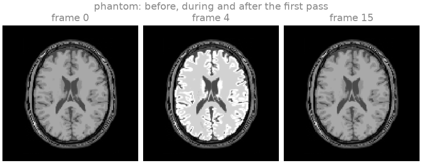
The phantom is the BrainWeb slice of the previous lessons with a contrast agent bolus passing through it. A gamma-variate curve describes the first-pass concentration over time, and each tissue enhances in proportion to its blood volume: strongly in grey matter, weakly in white matter, and not at all in cerebrospinal fluid. The series is therefore smooth in time, with the same anatomy in every frame, which is the structure the temporal penalty exploits.

CLASSES = {"grey matter": ("GM", 0.8), "white matter": ("WM", 0.25)}

Acquisition

FRAMES * SPOKES spokes are generated as one golden-angle trajectory and reshaped, so that the first axis indexes frames and the second the spokes within a frame. With \(\pi/2 \times 128 \approx 201\) spokes needed for a fully sampled frame, thirteen spokes undersample each frame by a factor of about fifteen. The image varies along the frame axis, so the operator holds one NUFFT per frame, all applied inside the same loop over the coils. The noise is that of the Cartesian lessons, of variance \(10^{-4}\) per sample.

trajectory = bt.traj(readout=SIZE, spokes=FRAMES * SPOKES, radial=True, golden=True)
trajectory = trajectory.reshape(FRAMES, SPOKES, SIZE, 3)


A = linop.NoncartesianSense(sensitivities, (FRAMES, SIZE, SIZE), traj=trajectory)
measured = bt.noise(A(series), n=1e-4, s=3)

print(f"{A.ishape} -> {A.oshape}")
print(A.plan)

(16, 128, 128) -> (8, 16, 13, 128)
Plan(transform=nufft, items=16, image=sensitivities, normal=kernel, coil_batch=1, streamed=coils, executor=slab)

plan.items is the number of frames the encoding carries, each with its own transform.

Reconstruction

Two reconstructions of the same data. The first treats the frames as independent: the adjoint of the encoding applied to density-compensated samples, which is the gridding reconstruction of thirteen spokes per frame, with the coils combined by the sensitivities. The second solves for the whole series at once, with a total-variation penalty along the frame axis: the solution is the series that explains all the data and changes least from frame to frame. The streak pattern of each frame is different, because each frame has different spokes, so it has a large temporal total variation and is suppressed, while the anatomy, which is the same in every frame, is not.

weights = torch.linalg.norm(trajectory.real[..., :2], dim=-1).clamp(min=0.25)
gridded = A.H(measured * weights.to(torch.complex64))

data = measured / optim.data_scaling(measured[..., None], A=A)
temporal = optim.ADMM(priors.TotalVariation(axes=(-3,), weight=0.02), maxiter=30)(data, A)

for name, volume in (("gridding", gridded), ("temporal TV", temporal)):
    print(f"{name:>12}  NRMSE over all frames {bt.nrmse(series.abs(), volume, scaled=True):.3f}")

   gridding  NRMSE over all frames 0.449
temporal TV  NRMSE over all frames 0.126

The frame axis is -3, the axis in front of the two spatial ones. A term given (-1, -2) would penalize the spatial gradient instead, and one given all three would penalize both; the axes a term acts on are the whole difference between a spatial and a temporal regularizer.

• 
• 

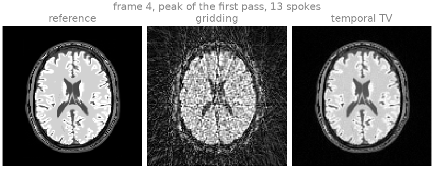
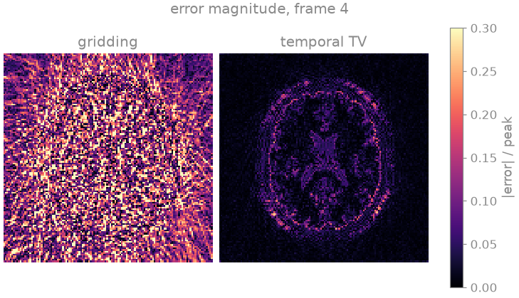
In the gridding reconstruction the streaks of thirteen spokes dominate the frame, and only the ventricles and the outline of the head are recognizable. The joint reconstruction recovers the anatomy and the enhanced cortex; its residual error is small and concentrated at the tissue boundaries, which carry the high spatial frequencies each frame samples most sparsely.

An x-t profile, one line of the image plotted against time, shows the time axis directly. The line below runs left to right through the ventricles and the grey matter on either side.

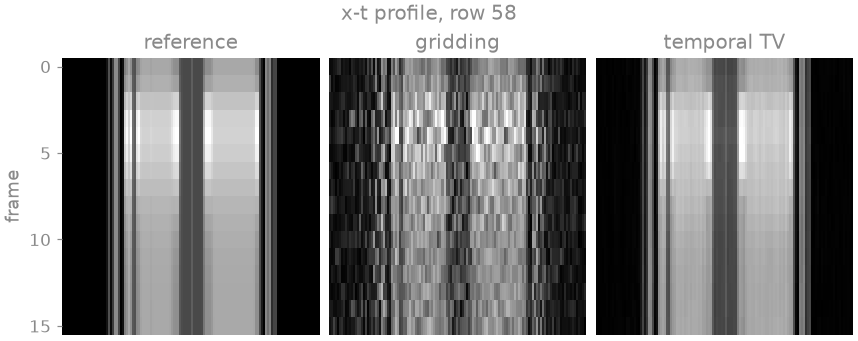
In the reference profile the grey matter brightens and fades over a few frames, while cerebrospinal fluid and the scalp stay constant. Gridding shows the same enhancement under a different streak pattern in every frame, so the profile changes from one row to the next even where the object does not; temporal total variation removes that variation and keeps the time course.

Time-intensity curve

A perfusion study reports the signal in a region as a function of time, so the reconstructions are compared on that curve too. The region is the grey matter, where the enhancement is strongest.

region = memberships[CLASS["GM"]] > 0.6

curves = {
    "reference": series.abs(),
    "gridding": scaled(gridded, series),
    "temporal TV": scaled(temporal, series),
}
truth = curves["reference"][:, region].mean(-1)
for name, volume in curves.items():
    if name == "reference":
        continue
    enhancement = volume[:, region].mean(-1)
    print(f"{name:>12}  curve NRMSE {float((enhancement - truth).norm() / truth.norm()):.3f}")

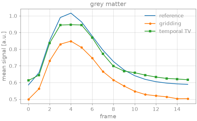
   gridding  curve NRMSE 0.153
temporal TV  curve NRMSE 0.039

Averaged over the grey matter, the streaks largely cancel, and gridding recovers the shape of the curve but not its level: part of the signal of each frame is spread into streaks across the field of view, outside the region. The joint reconstruction follows the reference curve closely, with the peak slightly attenuated and the baseline slightly raised: a temporal total-variation penalty flattens a signal change that lasts only a few frames more than any other feature, and a larger weight trades more of the peak for less noise.

References

[1]

Winkelmann S, Schaeffter T, Koehler T, Eggers H, Doessel O. An optimal radial profile order based on the Golden Ratio for time-resolved MRI. IEEE Trans Med Imaging 26(1):68-76 (2007). https://doi.org/10.1109/TMI.2006.885337

[2]

Feng L, Grimm R, Block KT, Chandarana H, Kim S, Xu J, Axel L, Sodickson DK, Otazo R. Golden-angle radial sparse parallel MRI: combination of compressed sensing, parallel imaging, and golden-angle radial sampling for fast and flexible dynamic volumetric MRI. Magn Reson Med 72(3):707-717 (2014). https://doi.org/10.1002/mrm.24980