Operators and solvers

This lesson rebuilds the reconstruction of the previous lessons from its parts – the encoding operator, the regularization term and the iterative algorithm – instead of calling a BART application, and shows that the result is identical.

bartorch.apps.pics() builds three objects and runs BART’s iteration with them: the SENSE encoding operator \(A = PFS\), the regularization terms, and the algorithm. Building them separately with bartorch.linop and bartorch.optim is what a reconstruction BART has no application for requires: an encoding with an additional factor, such as an off-resonance or motion-induced phase, a solver called from an outer loop, an operator defined in Python, or a gradient with respect to the data for training a network.

The example builds the Cartesian SENSE encoding of From k-space to image, checks it against the definition of the adjoint, solves with it, and compares the result with the application. The phantom, the coil sensitivities and the sampling are that example’s; the cell that builds them is hidden on this page and present in the script this page can be downloaded as.

Learning objectives

• Build bartorch.linop.CartesianSense and read the plan it was lowered into.

• Check an operator’s adjoint with the dot-product test.

• Prepare data as pics does and reproduce bartorch.apps.pics() bit for bit with bartorch.optim.FISTA.

• Compose operators, include one defined in Python, and differentiate through an application.

It follows Regularized reconstruction. The next section, Trajectories and transforms, uses these operators off the Cartesian grid.

import csv
from pathlib import Path

import brainweb_dl
import numpy as np
import torch
from brainweb_dl import get_mri

import bartorch
import bartorch.tools as bt
from bartorch import apps, linop, optim, priors

SIZE = 192
COILS = 8
ACCELERATION = 3
CALIBRATION = 24

The encoding operator

bartorch.linop.CartesianSense() is \(A = P F S\) as one operator. It takes the sensitivities, the shape of the image it maps from, and the sampling pattern; the shape of the k-space it maps to follows from those. bartorch.tools.pattern() reads the pattern off the measured data, as for a prospectively undersampled acquisition.

modulated=True selects BART’s uncentred sample convention, which its applications iterate in; the default is the centred convention that bartorch.fft() produces. The two differ by a modulation of the samples and give the same image, so the choice matters only when the operator is applied to data already in one of them, as it is below.

pattern = bt.pattern(kspace)
A = linop.CartesianSense(maps.squeeze(1), (SIZE, SIZE), pattern.squeeze(), modulated=True)

print(f"{A.ishape} -> {A.oshape}")
print(A.plan)
print(f"fused: {A.plan.fused}")

(192, 192) -> (8, 192, 192)
Plan(transform=fft, image=sensitivities, normal=transform, coil_batch=1, streamed=coils, executor=slab)
fused: True

A.plan reports the form the operator was lowered into: which transform, what multiplies the image and the samples, and how the normal operator \(A^H A\) is applied. It is a property of the built operator rather than a prediction, and plan.fused is false where the composition could not be expressed as one encoding and fell back to a chain, which computes the same numbers more slowly.

Applying the adjoint is not the same as applying the transpose, and a reconstruction built on the wrong one converges to the wrong image. The definition \(\langle Ax, y\rangle = \langle x, A^H y\rangle\) holds for any pair of vectors, and holds for random vectors as readily as for real data, so it is a usable check on an operator.

generator = torch.Generator().manual_seed(0)
probe = torch.randn(A.ishape, dtype=torch.complex64, generator=generator)
samples = torch.randn(A.oshape, dtype=torch.complex64, generator=generator)

forward = (A(probe).conj() * samples).sum()
adjoint = (probe.conj() * A.H(samples)).sum()
print(f"relative difference {abs(forward - adjoint) / abs(forward):.2e}")

relative difference 1.35e-07

Solving

A solver is called as solver(y, A). What it is given is not the array the scanner wrote but what pics iterates on: the sampling pattern applied, the modulation into the uncentred convention, and the data divided by the scaling bartorch.optim.data_scaling() estimates from the adjoint reconstruction, which is the step that makes a regularization weight transferable from one dataset to the next.

measured = bartorch.fftmod(kspace * pattern, axes=(-1, -2, -3), inverse=True)
scale = optim.data_scaling(measured)
data = (measured / scale).squeeze(1)

term = priors.Wavelet(axes=(-1, -2), weight=0.002)
assembled = optim.FISTA(term, maxiter=100)(data, A)

With the same preprocessing the assembled solve and the application are not merely close: they are the same iteration over the same operator, and return the same bits.

tool = apps.pics(kspace, maps, regularizers=term, solver="fista", maxiter=100)
print(f"identical to pics: {torch.equal(assembled.squeeze(), tool.squeeze())}")
print(f"NRMSE, adjoint {bt.nrmse(image.abs(), A.H(data).abs(), scaled=True):.3f}")
print(f"NRMSE, FISTA   {bt.nrmse(image.abs(), assembled.abs(), scaled=True):.3f}")

identical to pics: True
NRMSE, adjoint 0.119
NRMSE, FISTA   0.032

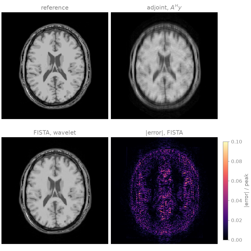
The adjoint of the encoding is not its inverse: \(A^H y\) is the sensitivity-weighted coil combination of the zero-filled k-space, and carries the aliasing of the undersampling and the shading of \(\sum_c |S_c|^2\), which the solve removes, as the NRMSE printed above shows. The error of the solution, at a tenth of the image peak, is concentrated at the tissue boundaries.

Operator algebra

@ composes, + adds, A.H is the adjoint and A.gram() the normal operator \(A^H A\). A composition builds a single BART operator rather than a Python chain, so a solver iterating on it does not return to Python between applications. bartorch.optim.maxeigen() runs the power iteration on an operator, which is how a gradient step size is chosen: the Lipschitz constant of the least-squares gradient is the largest eigenvalue of \(A^H A\).

print(f"largest eigenvalue of A^H A: {optim.maxeigen(A.gram()):.3f}")

largest eigenvalue of A^H A: 0.999

An operator defined in Python is composed with BART’s through from_callbacks(), which BART applies as a callback. Here it is a spatially varying phase, as an off-resonance or an eddy-current phase would be, placed between the image and the encoding.

field = torch.exp(1j * 0.4 * torch.pi * grid_x).to(torch.complex64)
phase = linop.LinearOperator.from_callbacks(
    (SIZE, SIZE), (SIZE, SIZE), lambda u: field * u, lambda u: field.conj() * u
)
composed = A @ phase
print(f"{composed.ishape} -> {composed.oshape}, fused: {composed.plan.fused}")

(192, 192) -> (8, 192, 192), fused: True

Differentiation

Applying an operator to a tensor that requires a gradient records the application for autograd. The gradient torch propagates back through \(y = Ax\) is \(A^H g\) rather than \(A^T g\), the conjugate Wirtinger convention torch uses for complex tensors. For a real \(A\), \(A^H = A^T\), so only a complex check distinguishes the two; Differentiation through reconstruction describes the backward passes of the solvers.

variable = data.new_zeros(A.ishape).requires_grad_(True)
residual = A(variable) - data
(residual.abs() ** 2).sum().backward()

expected = 2 * A.H(-data)
difference = float((variable.grad - expected).abs().max() / expected.abs().max())
print(f"relative difference from 2 A^H (Ax - y): {difference:.2e}")

relative difference from 2 A^H (Ax - y): 2.04e-07

The regularization terms are the subject of bartorch.priors, and the iterations of bartorch.optim; Inverse problems and their solvers states which algorithm applies to which problem.