Examples#
Reconstructions executed when the documentation is built, so every figure and printed number on these pages is produced by the code shown. The first six sections are a course read in order: each lesson states its aim and builds on the lessons before it. The tours are standalone. Every page can be downloaded as a Python script or a notebook, or opened in Colab. The concepts are in Explanation, and the interfaces in API reference.
Section |
Subject |
|---|---|
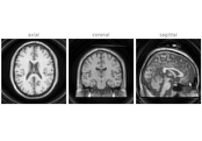
Tensors and BART’s dimensions, and a first reconstruction from undersampled Cartesian k-space |
|
Coil sensitivity estimation, nonlinear inversion, and noise prewhitening |
|
Tikhonov, wavelet and total-variation penalties, and the operator-and-solver form |
|
The NUFFT, density compensation, radial SENSE and dynamic golden-angle imaging |
|
Subspace \(T_1\) mapping, \(T_2\) estimation through a signal model, and maps from DICOM images |
|
Plug-and-play, unrolled and self-supervised networks, and uncertainty |
|
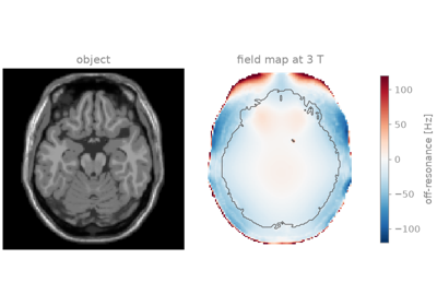
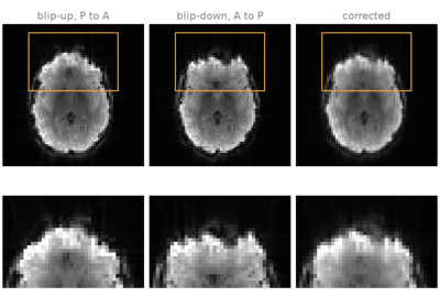
Corrections applied before and after a reconstruction |
The scripts need a built bartorch with its io extra, brainweb-dl, which downloads the
BrainWeb phantoms several examples build their images from, and
matplotlib and cmap for the figures:
pip install 'bartorch[io]' brainweb-dl matplotlib cmap
The learned-regularization section additionally requires lightning,
torchio, monai and deepinv, and the tours SimpleITK and
PyHySCO; each section page names what it needs.
Basics#
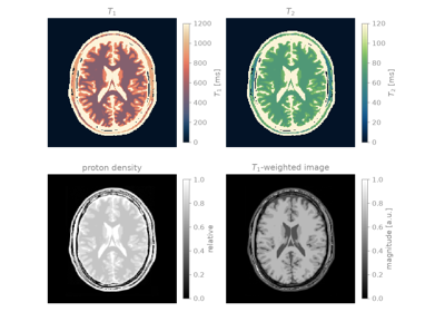
The course starts from the data a scanner delivers, multichannel k-space, and reconstructs an image from it. The first lesson relates PyTorch tensors to BART’s arrays and commands, simulates an acquisition with BART’s analytical phantom and verifies the centring and scaling of BART’s FFT against NumPy. The second reconstructs an undersampled Cartesian acquisition through the three steps every later section builds on: coil compression, calibration of the coil sensitivity maps by ESPIRiT, and a regularized SENSE reconstruction. The signal model is derived in The MRI encoding operator, and the array conventions are stated in Data layout and conventions.
Parallel imaging#
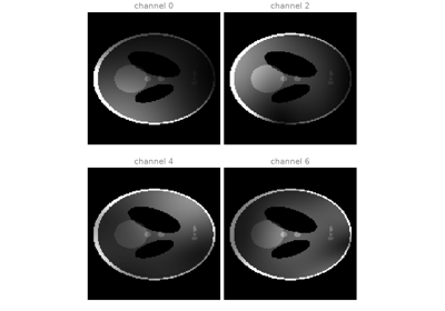
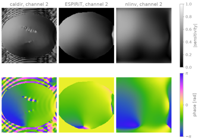
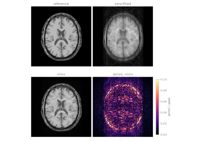
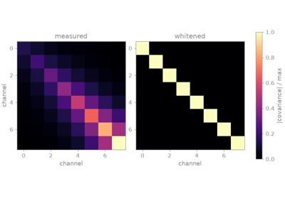
Parallel imaging recovers an image from k-space undersampled along the phase-encoding directions by exploiting the spatial sensitivities of a receive array. A SENSE reconstruction is only as accurate as its coil sensitivity maps, and it propagates the thermal noise of the channels, amplified by the g-factor. This section treats both: sensitivity estimation from the autocalibration (ACS) region, by direct division and by ESPIRiT; joint estimation of image and sensitivities by nonlinear inversion when the ACS region is too small for a separate calibration; and prewhitening of correlated channel noise, evaluated by the SNR of the reconstruction. The MRI encoding operator derives the SENSE model and Nonlinear forward models the joint estimation.
Regularization#
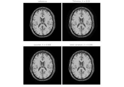
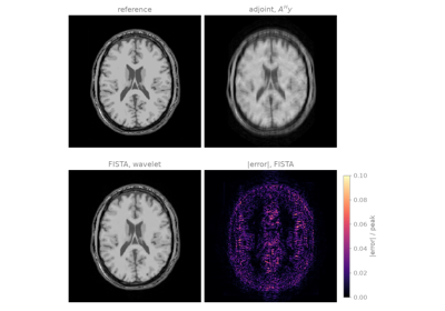
Beyond the acceleration factor the coil geometry supports, the SENSE problem is ill-conditioned: a least-squares solution amplifies noise, and the aliasing of the undersampling is not fully resolved. A regularized reconstruction adds prior knowledge of the image as a penalty. This section compares Tikhonov, wavelet-sparsity (compressed sensing) and total-variation penalties on one undersampled acquisition and shows how the regularization weight is chosen. It then writes the same reconstruction as an explicit encoding operator and an iterative solver, the form required by an encoding for which BART has no application. Inverse problems and their solvers introduces the formulations and the algorithms.
Non-Cartesian imaging#
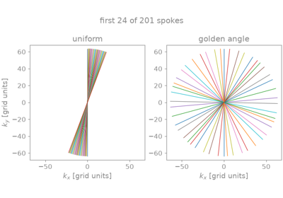
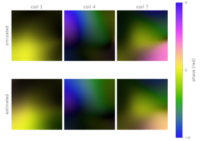
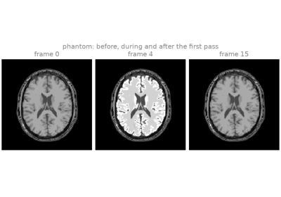
Radial and spiral trajectories sample k-space off the Cartesian grid. Their Fourier transform is a non-uniform FFT (NUFFT), their adjoint approximates an inverse only after density compensation, and the normal operator of an iterative reconstruction becomes a convolution with the point spread function of the trajectory. This section introduces trajectories, the NUFFT, density compensation and the point spread function; reconstructs an undersampled golden-angle radial acquisition by non-Cartesian SENSE, with coil sensitivities estimated from the radial data; and reconstructs a continuous golden-angle acquisition as a time series with a temporal regularizer. Non-Cartesian sampling defines the transform and its accuracy.
Model-based reconstruction#
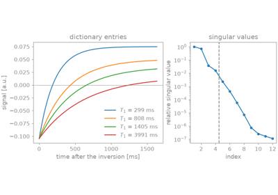
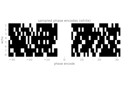
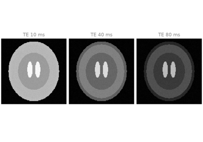
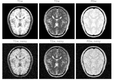
Quantitative MRI estimates tissue parameters such as \(T_1\) and \(T_2\) from a series of images acquired at different contrasts. Reconstructing each contrast separately and fitting a signal model afterwards ignores the relation between the contrasts that the signal model states. A model-based reconstruction places that relation in the forward operator, so that every contrast constrains the same unknowns. This section treats the two standard formulations: a linear subspace model, in which inversion-recovery signal curves are represented by a few temporal basis functions and \(T_1\) is fitted to the coefficient maps, and a nonlinear signal model, through which \(T_2\) maps are estimated directly from multi-echo k-space. Nonlinear forward models compares the two with reconstruction followed by a voxel-wise fit. The last lesson fits a signal model to magnitude images read from DICOM, as a scanner exports them, and writes the map back.
Learned regularization#
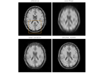
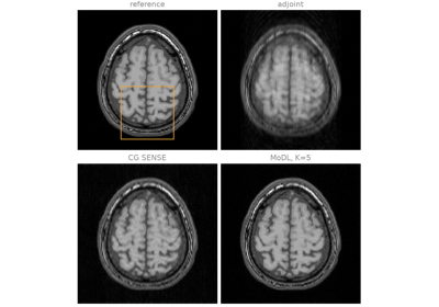
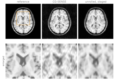
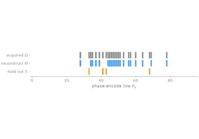
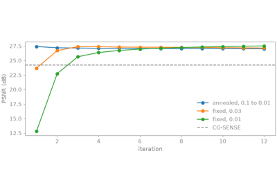
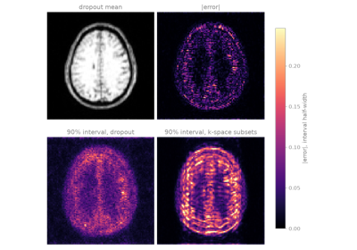
A learned reconstruction replaces the hand-specified regularization term by a neural network and keeps the encoding operator and the data consistency of the iterative reconstruction. This section starts with plug-and-play reconstruction, in which a pretrained denoiser takes the place of the proximal operator of ADMM and FISTA without any training, and proceeds to an unrolled network trained through BART’s ADMM (MoDL); networks for complex multi-contrast volumes, applied patch by patch; staged and self-supervised training of an unrolled network; plug-and-play with an annealed noise level; and calibrated voxel-wise uncertainty. Learned reconstruction describes where a network enters a reconstruction.
The section additionally requires:
pip install lightning torchio monai deepinv
The first lesson downloads the DRUNet weights deepinv distributes.
Tours#
Corrections applied to the data before reconstruction or to the image after it, each shown on its own and independent of the course: removal of readout oversampling and apodization, EPI Nyquist-ghost correction and regridding of ramp-sampled readouts, receive bias-field correction, correction of the geometric distortion caused by gradient nonlinearity, off-resonance deblurring of spiral images, rigid head-motion tracking from navigators, and correction of susceptibility distortion in EPI. The first six tours simulate the artefact from a known ground truth, so that the correction is evaluated against it; the seventh corrects measured data and evaluates the correction against an independent field map.
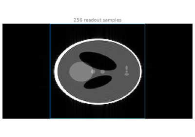
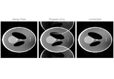
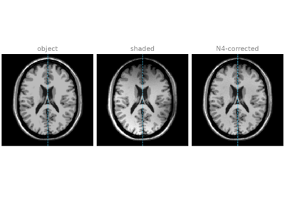
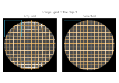
The first tour removes readout oversampling and compares Fermi and Hann apodization by their Gibbs ringing and resolution. The second corrects the Nyquist ghost of an EPI train from a three-line navigator and resamples a ramp-sampled readout. The third estimates the receive bias field of a head array with N4. The fourth corrects the geometric distortion and intensity error of gradient nonlinearity from the coil’s spherical-harmonic coefficients. The fifth deblurs a spiral image off resonance by multifrequency interpolation and by a time-segmented reconstruction. The sixth measures rigid head motion from three orthogonal navigator planes and filters it across a scan. The seventh corrects the susceptibility distortion of a 3 T EPI pair with reversed phase encoding, downloaded from OpenNeuro.
The section additionally requires the following packages, and the seventh tour
downloads about 2 MB of data into ~/.cache/bartorch-examples:
pip install SimpleITK PyHySCO