1. Your data as tensors

If you have used BART before, you know its arrays as CFL files on disk and its commands as programs you call from a shell. bartorch runs the same BART inside your Python process: every command is a Python function that takes and returns torch.Tensor objects, with no files and no subprocess in between. In this lesson you see what your data look like on that side: how a multichannel image and its k-space are laid out as tensors, which Fourier transform takes one to the other, and how a BART command line maps onto a function call.

Every later lesson relies on these conventions. A reconstruction that is off by a factor of \(\sqrt{N}\), or shifted by half a voxel because the k-space centre is misplaced, usually results from misreading one of them.

Learning objectives

• Read a tensor shape as BART’s dimension vector, and find the receive-channel axis in it.

• Make a phantom as an image, as coil images and as analytical k-space.

• Know where bartorch.fft() puts the k-space centre and how it normalizes, and check both against numpy.fft.fftn().

• See why analytical k-space, cut to the acquired matrix, reconstructs with Gibbs ringing.

• Call a BART command from Python, and the same command from its command line.

Next: 2. From k-space to an image, where you reconstruct an undersampled scan with the functions you meet here.

A multichannel image

BART stores an array in Fortran order and describes it by a dimension vector whose first entry varies fastest: readout (x), then the phase-encoding directions (y, z), then the receive channels in BART’s dimension 3, then further dimensions for sets of maps, echoes, frames and so on. A torch tensor holding the same bytes in C order has the reversed shape, so no copy is made between the two. A 2D multichannel image is therefore (coils, 1, y, x): the 1 is BART’s z, and the readout is the last axis. Data layout lists the layouts you meet in the rest of the course.

bartorch.tools.phantom() is BART’s phantom command. On its own it gives you the Shepp-Logan image; with coils it gives you that image as seen by each channel of BART’s analytical eight-channel head coil.

import numpy as np
import torch

import bartorch
import bartorch.tools as bt

SIZE = 128
COILS = 8

image = bt.phantom(SIZE)
coil_images = bt.phantom(SIZE, coils=COILS)

print(f"image {tuple(image.shape)}, {image.dtype}")
print(f"coil images {tuple(coil_images.shape)}")
print(f"as BART sees them {list(reversed(coil_images.shape))}")

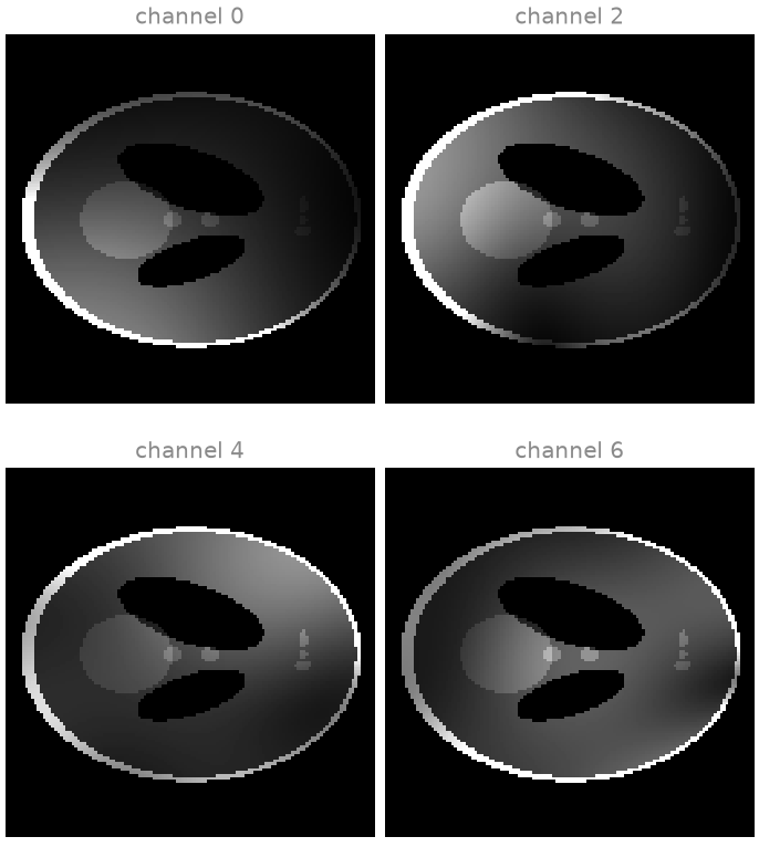
image (128, 128), torch.complex64
coil images (8, 1, 128, 128)
as BART sees them [128, 128, 1, 8]

Each channel sees the object through its own sensitivity: bright next to its coil element, dark on the far side of the head. The channel axis, first in the tensor shape, is BART’s dimension 3, the fourth entry of the reversed shape.

Combining the channels

The usual way to make one magnitude image from a receive array is the root sum of squares (RSS) over the channels, \(\sqrt{\sum_c |x_c|^2}\). bartorch.rss() takes the channel axis as a tensor axis, as every function in bartorch does, rather than as BART’s bitmask:

combined = bartorch.rss(coil_images, axes=(0,))
print(f"combined {tuple(combined.shape)}")

combined (1, 128, 128)

Fourier transform

What a channel measures is the Fourier transform of its coil image, sampled on the k-space grid. bartorch.fft() is BART’s centred transform: the k-space centre (DC) and the image centre both sit at index n // 2, which is how scanners deliver k-space and how you display it. It is unnormalized unless you ask for unitary=True.

kspace = bartorch.fft(coil_images, axes=(-2, -1), unitary=True)

You can check this against NumPy. For an even matrix size, the centred transform is NumPy’s transform between an ifftshift and an fftshift:

shifted = np.fft.ifftshift(coil_images.numpy(), axes=(-2, -1))
reference = np.fft.fftshift(
    np.fft.fft2(shifted, norm="ortho"),
    axes=(-2, -1),
)

difference = np.abs(kspace.numpy() - reference).max() / np.abs(reference).max()
ratio = float(coil_images.norm() / kspace.norm())
print(f"largest difference, relative to the peak: {difference:.1e}")
print(f"norm ratio image / k-space: {ratio:.6f}")

largest difference, relative to the peak: 1.7e-07
norm ratio image / k-space: 1.000004

The two transforms differ by single-precision round-off. The unitary transform keeps the \(\ell_2\) norm (Parseval’s theorem), which is why the norm ratio is one: white noise has the same standard deviation in k-space as in the image.

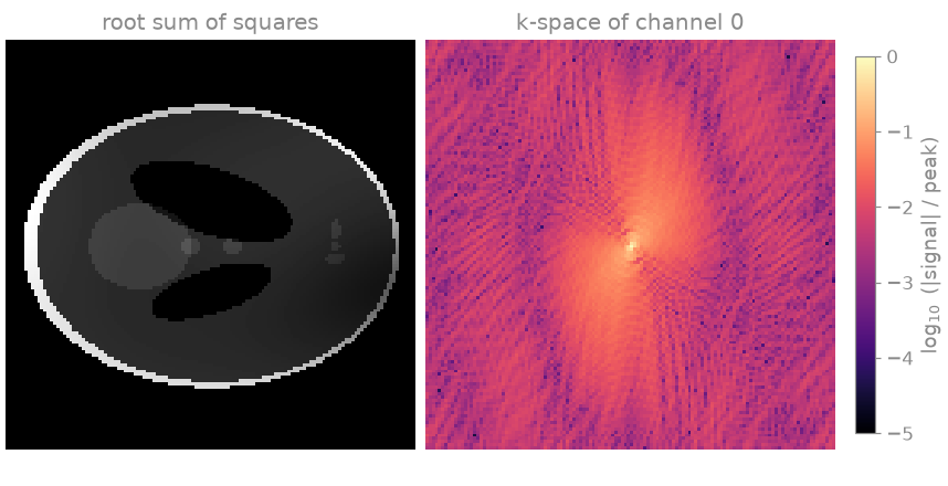
On the left is the RSS image, with the shading the summed coil sensitivities leave on it. On the right is the k-space of one channel, on a logarithmic scale. It spans five orders of magnitude: most of the energy is at the centre, which sets the contrast, while the periphery carries the edges and the fine detail. This is what variable-density undersampling exploits in lesson 2.

Analytical k-space

The k-space above is the discrete transform of a sampled image, so transforming it back gives you that image exactly. A scanner does not measure that. It measures the continuous object, whose spectrum never ends, and keeps only the part inside \(\pm k_{\max}\). kspace=True asks phantom for exactly that: the Fourier transform of its ellipses, evaluated analytically at the sample positions. Simulating data with the same discrete model you then invert is the inverse crime [1]; analytical k-space avoids it, and is the more realistic test data.

analytical = bt.phantom(SIZE, kspace=True)
truncated = bartorch.ifft(analytical, axes=(-2, -1))

error = float((truncated - image).norm() / image.norm())
print(f"relative difference from the sampled phantom: {error:.3f}")

• 
• 

relative difference from the sampled phantom: 0.218

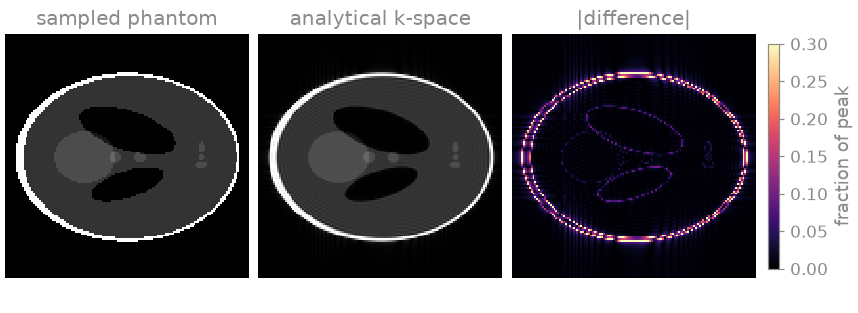
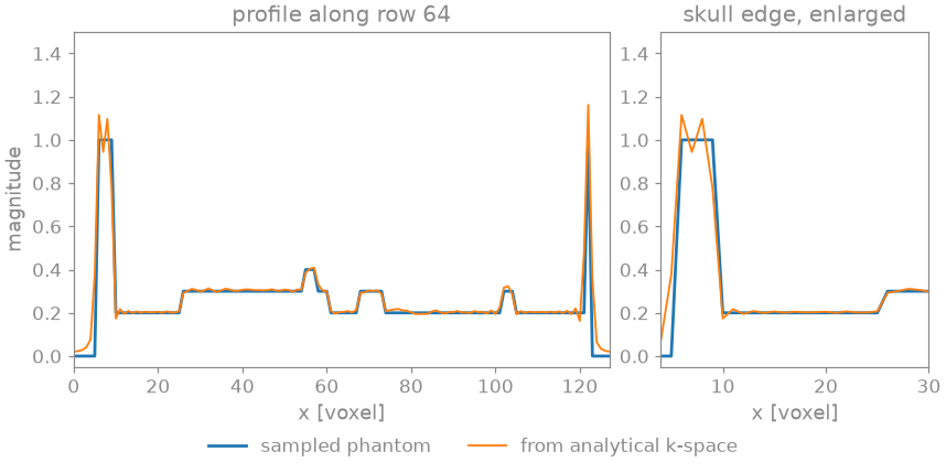
The difference is largest at the edges of the ellipses and fades away from them. The profile through the centre shows the ringing itself: the image from analytical k-space overshoots at every step in intensity and oscillates next to it with a period of about two voxels. That is the truncation artefact you see next to sharp edges on a scanner.

Here you use the unnormalized inverse, because phantom scales its k-space so that the unnormalized inverse returns the image’s intensities.

The command line

A function of bartorch.tools takes BART’s options as keyword arguments, under their long names or their single-letter flags, and reverses the shape of every tensor it hands to BART. The bartorch console command takes BART’s own command lines and works on CFL files, so a script written for the bart executable runs against the same library. bartorch.cli.main() runs one such command line in your process. bartorch.io.writecfl() wants the array in BART’s order, which is the transpose of a C-order array:

import tempfile

from pathlib import Path

with tempfile.TemporaryDirectory() as directory:
    source = str(Path(directory) / "coils")
    target = str(Path(directory) / "kspace")
    bartorch.io.writecfl(source, coil_images.numpy().T)
    status = bartorch.cli.main(["fft", "-u", "3", source, target])
    from_files = torch.as_tensor(bartorch.cli.read(target))

print(f"exit status {status}")
print(f"identical to bartorch.fft: {torch.equal(from_files, kspace)}")

exit status 0
identical to bartorch.fft: True

-u asks for the unitary transform, and 3 is BART’s bitmask for its dimensions 0 and 1 (readout and the first phase encoding), which are the last two tensor axes. Both routes run the same BART function on the same bytes, so the results are identical, bit for bit.

One difference matters later. A BART command is not recorded by autograd, so its result has no gradient with respect to its inputs. The operators of bartorch.linop and the solvers of bartorch.optim, which you meet in lesson 6 (6. Custom encoding and solver), are differentiable. Execution model describes both routes.

Exercise: matrix size

Does acquiring more of k-space get rid of the ringing? Repeat the comparison with analytical k-space at a few matrix sizes:

sizes = (64, 128, 256, 512)
errors, overshoots = [], []
for n in sizes:
    sampled = bt.phantom(n)
    from_kspace = bartorch.ifft(bt.phantom(n, kspace=True), axes=(-2, -1))
    errors.append(float((from_kspace - sampled).norm() / sampled.norm()))
    overshoots.append(float(from_kspace.abs().max() / sampled.abs().max()))

for n, e, o in zip(sizes, errors, overshoots):
    print(f"{n:>4}: relative difference {e:.3f}, peak {o:.2f} x the phantom's")

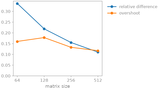
 64: relative difference 0.336, peak 1.16 x the phantom's
128: relative difference 0.218, peak 1.18 x the phantom's
256: relative difference 0.155, peak 1.13 x the phantom's
512: relative difference 0.110, peak 1.12 x the phantom's

The relative difference falls by about \(\sqrt{2}\) for every doubling of the matrix: the ringing occupies a band of a few voxels along each edge, a shrinking fraction of the image. The overshoot does not decrease: the brightest voxel stays more than a tenth above the phantom’s peak at every size. This is the Gibbs phenomenon: truncating the spectrum of an object with discontinuities produces an overshoot at each of them, whatever the matrix size. Try multiplying the analytical k-space by a Hann window along both axes before the inverse, and see which of the two numbers changes.

As a spec

What this lesson built, stated the way you would ask an agent for it:

With bartorch, make BART's 128x128 Shepp-Logan phantom as an image and as
8 coil images (bt.phantom, shape (coils, 1, y, x)), combine the channels
with bartorch.rss over axis 0, and transform them to k-space with
bartorch.fft over the last two axes, unitary. Check the transform against
numpy's fft2 between ifftshift and fftshift (norm="ortho"). Reconstruct
analytical k-space (bt.phantom(kspace=True)) with the unnormalized
bartorch.ifft and report its relative difference from the sampled
phantom. Finally run "fft -u 3" through bartorch.cli.main on CFL files
and check the result equals bartorch.fft's.

References

[1]

Guerquin-Kern M, Lejeune L, Pruessmann KP, Unser M. Realistic analytical phantoms for parallel magnetic resonance imaging. IEEE Trans Med Imaging 31(3):626-636 (2012). https://doi.org/10.1109/TMI.2011.2174158