Gradient nonlinearity

Spatial encoding assumes that every gradient field changes linearly with position. A real gradient coil departs from that more and more with the distance from isocentre, so each spin is encoded at a position displaced from its true one. The image is warped, by a few millimetres at the edge of a head-sized field of view and by centimetres at the edge of a body-sized one, and the voxel volume changes with the warp. The displacement is a property of the coil: the manufacturer states it as the coefficients of a spherical-harmonic expansion of each gradient field [1]. To correct it you evaluate that expansion at every voxel and resample the image at the positions where the voxels were actually encoded.

In this tour you warp a grid phantom in a coronal slice over a 450 mm field of view with a coil described by third-order harmonics, and correct it with bartorch.tools.Gradunwarp. The coil is a generic one, defined in the code; no manufacturer’s table is used.

Prerequisites: lesson 1, 1. Your data as tensors.

Learning objectives

• Describe a gradient coil’s nonlinearity by its spherical-harmonic coefficients with GradientCoefficients.

• Relate the displacement to the distance from isocentre and to the gradient axis.

• Correct the geometry and the intensity of an image with Gradunwarp, and tell the two apart.

• Place an image in scanner coordinates by its orientation and field of view.

import numpy as np
import torch

import bartorch.tools as bt

The coil

GradientCoefficients holds the cosine and sine coefficients \(\alpha_{nm}\) and \(\beta_{nm}\) of each gradient field’s departure from linearity, in the Siemens convention: harmonics normalized over a reference radius \(R_0\), and positions in scanner coordinates, with \(z\) along the bore. An all-zero table is a perfectly linear coil.

Each gradient field is odd along its own axis, so its lowest-order nonlinear terms are of third order: \(\alpha_{31}\) for the \(x\) gradient, \(\beta_{31}\) for the \(y\) gradient and \(\alpha_{30}\) for the \(z\) gradient, whose harmonic is proportional to \(z\,(2z^2 - 3x^2 - 3y^2)\). The signs and sizes of the terms decide where the image is compressed and where it is stretched. On a short whole-body coil the \(z\) gradient is usually the least linear, so you give it the largest term:

ORDER = 3
alpha = np.zeros((3, ORDER + 1, ORDER + 1))
beta = np.zeros_like(alpha)
alpha[0, 3, 1] = -0.04  # x gradient
beta[1, 3, 1] = -0.04  # y gradient
alpha[2, 3, 0] = -0.06  # z gradient
coil = bt.GradientCoefficients(
    basis="normalized", alpha=alpha, beta=beta, reference_radius_mm=250.0
)

The slice

The correction needs to know where each voxel sits in the scanner. Your slice is coronal through isocentre, 256 x 256 over a 450 mm field of view (1.8 mm voxels): rows run from superior to inferior along \(-z\), and columns from right to left along \(x\). The orientation matrix says, for each array axis, along which scanner direction it increases: its columns are the row axis and the column axis, its rows are \(x\), \(y\) and \(z\).

SIZE, FOV_MM = 256, 450.0
VOXEL_MM = FOV_MM / SIZE
coronal = np.array([[0.0, 1.0], [0.0, 0.0], [-1.0, 0.0]])
unwarp = bt.Gradunwarp(
    coil,
    shape=(SIZE, SIZE),
    fov_mm=(FOV_MM, FOV_MM),
    orientation=coronal,
)

Gradunwarp evaluates the expansion at every voxel of the corrected grid. Its source_grid is the index into the acquired image at which each voxel was encoded, so the displacement is the difference from the voxel’s own index:

grid = np.meshgrid(np.arange(SIZE), np.arange(SIZE), indexing="ij")
index = np.stack(grid, axis=-1)
displacement_mm = (unwarp.source_grid - index) * VOXEL_MM
offset_mm = (index - (SIZE - 1) / 2) * VOXEL_MM

100 mm from isocentre: displacement  0.9 mm along z,  0.5 mm along x
150 mm from isocentre: displacement  3.3 mm along z,  1.8 mm along x
200 mm from isocentre: displacement  7.6 mm along z,  4.1 mm along x

The displacement grows with the cube of the distance from isocentre: under a millimetre at 100 mm, several at 200 mm, and about twice as large along \(z\) as along \(x\), as the coefficients say it should be.

The acquisition

The object is a grid phantom: a disc 420 mm across carrying lines 30 mm apart, written in closed form so that you can evaluate it at any position. The acquired image at index \(p\) holds the object at the position \(r\) encoded there, the solution of \(r + d(r) = p\), found by fixed-point iteration. Its intensity is divided by the Jacobian determinant of the mapping, because a voxel whose volume the nonlinearity enlarges collects the signal of a larger region. That code simulates the artefact rather than correcting it, so it is hidden; acquired is the warped image and truth the object on the true grid.

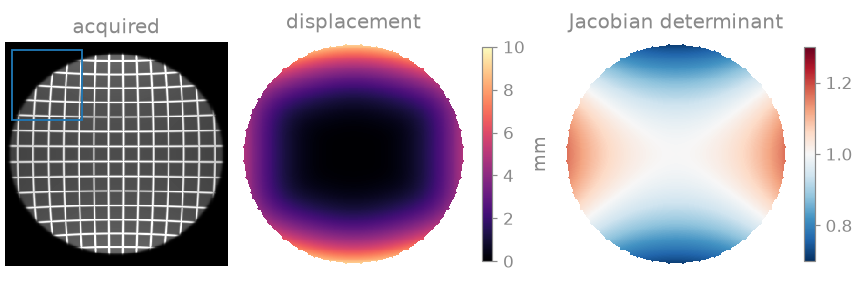
The centre of the field of view is untouched, and the displacement rises towards the edge, fastest at the top and bottom, along \(z\). There the Jacobian determinant is below one: the image is compressed towards isocentre, each voxel collects the signal of a larger region, and the periphery comes out brighter. Along \(x\) the image is stretched and darker. Off the axes the \(z\) displacement follows its harmonic and changes sign where \(2z^2 = 3x^2\), which is the cross you see in the Jacobian determinant.

The correction

Calling the Gradunwarp on an image resamples it at the source grid by cubic B-spline interpolation and multiplies it by the Jacobian determinant, which restores the intensity. With jacobian=False it corrects the geometry only, which lets you see the two parts separately:

image = torch.as_tensor(acquired, dtype=torch.float32)
corrected = unwarp(image).numpy()

geometry = bt.Gradunwarp(
    coil,
    shape=(SIZE, SIZE),
    fov_mm=(FOV_MM, FOV_MM),
    orientation=coronal,
    jacobian=False,
)
geometry_only = geometry(image).numpy()

• 
• 
• 
• 

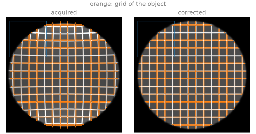
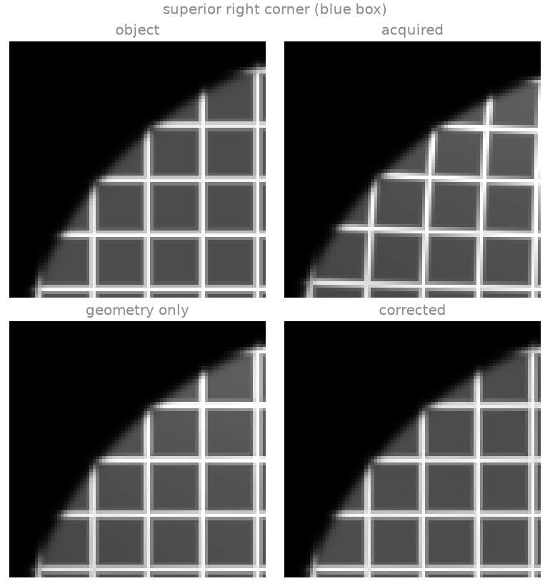
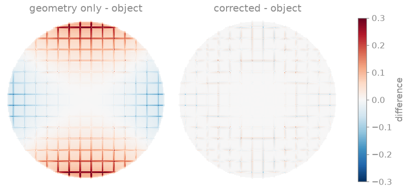
acquired       NRMSE 0.427
geometry only  NRMSE 0.118
corrected      NRMSE 0.025

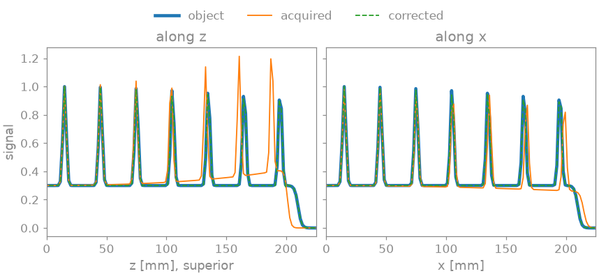
In the acquired image the grid lines bend away from the grid of the object (orange) towards the edge; after correction they lie on it. In the enlarged corner the geometry-only correction already puts the lines back in place, but leaves the intensity error of the Jacobian: its difference from the object is positive (red) at the top and bottom and negative (blue) at the sides. The full correction removes both, and the NRMSE against the object drops from the acquired image’s to a few per cent. What is left is the error of interpolating the acquired image, largest on the thin lines where compression has undersampled them. The profiles show the same thing on the two axes: the acquired lines move inwards and brighten along \(z\), move outwards along \(x\), and the corrected lines sit on the object’s.

For a real coil, from_file() reads the manufacturer’s table, and from_mrd() and from_affine() take the geometry of the image from an MRD header or an affine. Scanners apply a two-dimensional correction in the plane of the slice by default; the through-plane displacement moves signal between slices, and correcting it needs the whole volume.

Exercise: coil nonlinearity

The displacement is linear in the coefficients. Scale the \(z\) gradient’s term and see how far a voxel 200 mm above isocentre moves:

for term in (-0.03, -0.06, -0.12):
    stronger = alpha.copy()
    stronger[2, 3, 0] = term
    trial = bt.Gradunwarp(
        bt.GradientCoefficients(
            basis="normalized",
            alpha=stronger,
            beta=beta,
            reference_radius_mm=250.0,
        ),
        shape=(SIZE, SIZE),
        fov_mm=(FOV_MM, FOV_MM),
        orientation=coronal,
    )
    moved_mm = (trial.source_grid - index) * VOXEL_MM
    along_z, _ = displacement_at(moved_mm, offset_mm, 200)
    print(f"alpha_30 = {term:+.2f}: {along_z:4.1f} mm at z = 200 mm")

alpha_30 = -0.03:  3.8 mm at z = 200 mm
alpha_30 = -0.06:  7.6 mm at z = 200 mm
alpha_30 = -0.12: 15.2 mm at z = 200 mm

Doubling the coefficient doubles the displacement. Try a positive sign as well, and look at which way the grid lines move.

As a spec

What this tour built, stated the way you would ask an agent for it:

Correct the gradient-nonlinearity distortion of a 2D coronal slice
(256 x 256, 450 mm field of view, rows superior to inferior along -z,
columns along +x) with bt.Gradunwarp. Describe the coil with
bt.GradientCoefficients (normalized basis, R0 250 mm, third-order
alpha_31 for x, beta_31 for y, alpha_30 for z). Apply the full
correction and a geometry-only one (jacobian=False), report the NRMSE of
each against the object, and the displacement in mm at 100, 150 and
200 mm from isocentre along z and x.

References

[1]

Janke A, Zhao H, Cowin GJ, Galloway GJ, Doddrell DM. Use of spherical harmonic deconvolution methods to compensate for nonlinear gradient effects on MRI images. Magn Reson Med 52(1):115-122 (2004). https://doi.org/10.1002/mrm.20122