Subspace-constrained T1 mapping

In this tour you estimate a \(T_1\) map from a single continuous inversion-recovery acquisition in which each of four hundred time points is encoded by one radial spoke, so each frame on its own is undersampled about two-hundredfold. The recovery curves of all plausible \(T_1\) values span a subspace of low dimension; reconstructing the few coefficients of that subspace instead of the individual frames reduces the number of unknowns by two orders of magnitude.

The sequence is an inversion pulse followed by a train of spoiled gradient echoes with a small flip angle, each echo read out along one golden-angle spoke, as in MPnRAGE and radial Look-Locker methods. After the inversion the longitudinal magnetization recovers towards a steady state at an apparent rate that depends on \(T_1\), the flip angle and the repetition time, so every voxel follows one of a family of recovery curves. You simulate that family as a dictionary, and its dominant singular vectors \(\Phi\) are the basis of the subspace [1]. The time series is then \(x_t = \sum_a \Phi_{at} \alpha_a\), and the basis enters the encoding on the k-space side, between the transform of each frame and its samples:

\[y[c, t] = \sum_a \Phi_{at} \, \mathrm{NUFFT}_t \!\left( S_c \, \alpha_a \right).\]

You reconstruct the coefficient maps \(\alpha_a\) under a total-variation penalty, synthesize any frame of the series from them, and estimate \(T_1\) by matching each voxel’s coefficients against the dictionary. Where lesson 9 fits a nonlinear model directly to k-space, here the model is linear and only constrains the series; the dynamic series of Dynamic golden-angle radial MRI is constrained by a penalty instead.

Prerequisites: lessons 8 and 9, 8. Radial SENSE and 9. Nonlinear inversion for T2 mapping.

Learning objectives

• Simulate a dictionary of inversion-recovery curves and extract a low-dimensional subspace from it by the singular value decomposition.

• Include a subspace basis in a non-Cartesian encoding.

• Reconstruct coefficient maps under a total-variation penalty, and synthesize images at any inversion time from them.

• Estimate \(T_1\) by dictionary matching in the subspace, compare it with matching frames reconstructed one at a time, and recognise the partial-volume bias of a voxelwise fit.

The dictionary and its subspace

The dictionary is simulated from the sequence that is played, one curve per \(T_1\). MPnRAGESimulator is that sequence, an inversion followed by a spoiled gradient-echo train with every shot read, and simulate evaluates it over an array of parameters at once, giving (entries, frames). Handed to bartorch.nlop.Bloch(), the same object is a model operator, which is how lesson 9 solves for the maps directly; here you only need its forward evaluation.

The basis is the first RANK left singular vectors of the dictionary, one row per coefficient.

import torch

import bartorch
import bartorch.tools as bt

from bartorch import linop, optim, priors
from blochsim.simulators import MPnRAGESimulator

COILS = 8
FRAMES = 400
RANK = 4

TR = 4.1  # ms
FLIP = 6.0  # degrees

t1_values = torch.linspace(100.0, 4500.0, 200)  # ms

sequence = MPnRAGESimulator(nshots=FRAMES, flip=FLIP, TR=TR)
dictionary = torch.as_tensor(sequence.simulate(T1=t1_values))

atoms = dictionary.T.to(torch.complex64)  # (frames, entries)
left = torch.linalg.svd(atoms, full_matrices=False)[0]
basis = left[:, :RANK].T.contiguous()  # (RANK, frames)

print(f"dictionary {tuple(dictionary.shape)}, basis {tuple(basis.shape)}")

dictionary (200, 400), basis (4, 400)

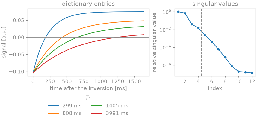
On the left are a few entries of the dictionary. The signal starts negative after the inversion, passes through zero at a time that grows with \(T_1\), and approaches the steady state of the gradient-echo train. The curves are smooth and similar, so a few singular vectors represent all of them: on the right, the fourth singular value is below 2 % of the first and the twelfth below \(10^{-6}\) of it. The dashed line marks the rank you use, four. The rank is a modelling decision. Too few coefficients bias the recovered curves towards the span of the basis; too many add unknowns that the undersampled data have to determine.

The object

The object is the BrainWeb slice [7] of the course lessons. Each tissue class gets the \(T_1\) of the BrainWeb table and its own curve from the same signal model, and the series is the membership-weighted sum of them. A voxel holding two tissues therefore follows a sum of two recovery curves, which is not itself an inversion-recovery curve: that is the partial-volume error any voxelwise fit carries. The code that builds the series is hidden.

Acquisition

You play one golden-angle spoke per repetition time, four hundred of them in 1.64 s after the inversion. Each frame is sampled by a single spoke, about \(1/200\) of what a fully sampled frame needs; together, the spokes of the train cover k-space densely. The trajectory indexes frames as well as samples, so you reshape it to (frames, 1, readout, 3). The coils are BART’s eight-channel head coil, normalized as in lesson 2, and the noise has a variance of \(10^{-5}\) per sample; printed below is what that means as the signal-to-noise ratio of white matter in a fully sampled image of the steady state.

trajectory = bt.traj(
    readout=SIZE,
    spokes=FRAMES,
    radial=True,
    golden=True,
)
trajectory = trajectory.reshape(FRAMES, 1, SIZE, 3)

sensitivities = bt.coils(t=bt.grid(D=(SIZE, SIZE, 1)), n=COILS)[:, 0]
sensitivities /= bartorch.rss(sensitivities, axes=(0,), keepdim=True)

frames = linop.NoncartesianSense(
    sensitivities,
    (FRAMES, SIZE, SIZE),
    traj=trajectory,
)
measured = bt.noise(frames(series), n=1e-5, s=5)

white-matter SNR of a fully sampled steady-state image: 15

frames is the encoding of the four hundred frames, which is how you simulated the data. For the reconstruction you build the same encoding with basis: its image is the four coefficient maps rather than the four hundred frames, and the basis contracts the one into the other on the k-space side.

A = linop.NoncartesianSense(
    sensitivities,
    (RANK, SIZE, SIZE),
    traj=trajectory,
    basis=basis,
)
print(f"{A.ishape} -> {A.oshape}")
print(A.plan)

(4, 128, 128) -> (8, 400, 1, 128)
Plan(transform=nufft, image=sensitivities, kspace=basis, contraction=subspace(4), normal=kernel, coil_batch=1, streamed=coils, executor=slab)

plan.contraction reports the subspace and its rank. The normal operator is a point spread function over the basis as well as the trajectory, so an iteration never transforms the four hundred frames.

Reconstruction

You penalize the total variation [2] of each coefficient map over the two spatial axes. A tissue follows one recovery curve throughout, so its coefficients are piecewise constant; the noise, which the data determine least well in the coefficients of the weaker singular vectors, is not. A locally low-rank penalty [3] over blocks of voxels is the other common choice. A block that straddles two tissues is rank two, though, and shrinking its second singular value mixes their curves and biases the fitted \(T_1\) towards the neighbouring tissue.

The ADMM penalty parameter rho weights the auxiliary variable, which starts at zero, against the data in each update of the coefficients. At the default of 0.5, the coefficients of the weaker singular vectors, which carry the differences between recovery curves, are still biased towards zero after forty iterations, and the fitted \(T_1\) with them. With 0.05 the data determine them within that number of iterations.

data = measured / optim.data_scaling(measured[..., None], A=A)
term = priors.TotalVariation(axes=(-1, -2), weight=0.001)
coefficients = optim.ADMM(term, maxiter=40, rho=0.05)(data, A)

# The series at every time point, from its coefficients.
recovered = torch.einsum("af,ayx->fyx", basis, coefficients)

For comparison, you also reconstruct the frames one at a time: the density-compensated adjoint of the encoding without the basis, which is gridding of each frame from its single spoke.

density = torch.linalg.norm(trajectory.real[..., :2], dim=-1).clamp(min=0.25)
gridded = frames.H(measured * density.to(torch.complex64))

for name, estimate in (("frame by frame", gridded), ("subspace", recovered)):
    nrmse = bt.nrmse(series.abs(), estimate.abs(), scaled=True)
    print(f"{name:>14}: NRMSE of the series {nrmse:.3f}")

frame by frame: NRMSE of the series 1.621
      subspace: NRMSE of the series 0.145

Dictionary matching

You match the recovered coefficients against the dictionary projected onto the same subspace, by the normalized inner product: dictionary matching in four dimensions rather than four hundred. Matching in the subspace and matching the reconstructed curves differ only by the component of the dictionary that the basis discards. The frame-by-frame series has no subspace, so you match it against the dictionary itself.

def match(voxels, atoms):
    """The T1 of the atom with the largest normalized inner product."""
    voxels = voxels.reshape(len(atoms), -1)
    voxels = voxels / voxels.norm(dim=0, keepdim=True).clamp(min=1e-12)
    atoms = atoms / atoms.norm(dim=0, keepdim=True)
    best = (atoms.conj().T @ voxels).abs().argmax(0)
    return t1_values[best].reshape(SIZE, SIZE)


t1_map = match(coefficients, basis @ atoms)
t1_gridded = match(gridded, atoms)

                 table  frame by frame  subspace   [ms]
          CSF     2569            2289      2598   (68 voxels)
           GM      833             852       830   (76 voxels)
           WM      500             520       498   (1143 voxels)
  MUSCLE/SKIN      900             896       896   (22 voxels)
frame by frame  mean relative T1 error: interior 0.057, whole head 0.099;  white-matter standard deviation 29 ms
      subspace  mean relative T1 error: interior 0.012, whole head 0.092;  white-matter standard deviation 6 ms

The table gives the median fitted \(T_1\) in the interior of each tissue class, the voxels one class dominates less a one-voxel rim, so that the numbers are not those of partial volume; the two lines below it average the relative error over those interiors and over the whole head. The figures below show the coefficient maps first, then the series and the \(T_1\) maps.

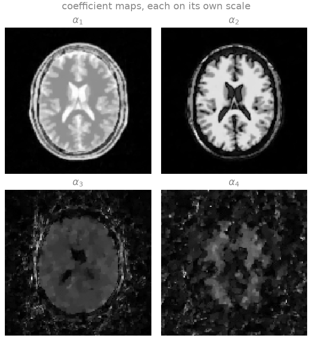
Each coefficient map is the weight of one singular vector of the dictionary. The first looks like a proton-density-weighted image, because the first singular vector is close to the mean recovery curve. The later ones encode the differences between the curves of short and long \(T_1\), and are not images of any tissue contrast. The basis is orthonormal, so the noise is spread over the four maps alike while the signal falls with the singular value: the fourth map has the lowest signal-to-noise ratio of the four.

Synthetic inversion-time images

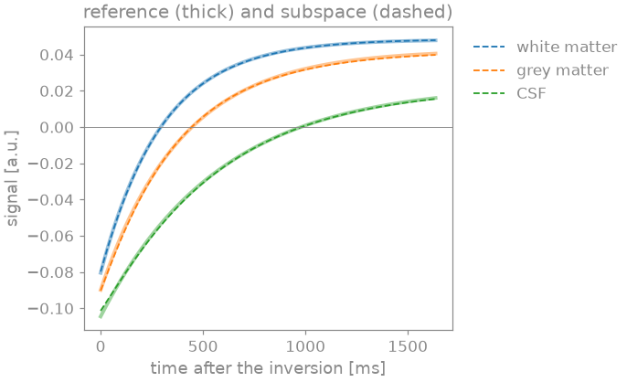
The coefficient maps determine the whole series: multiplying by the basis gives you the image at every one of the four hundred time points, each of which was measured with a single spoke. Early after the inversion the longitudinal magnetization is negative in every tissue; each tissue then passes through zero at its own null time, shortest for white matter, and approaches the steady state of the gradient-echo train.

• 
• 

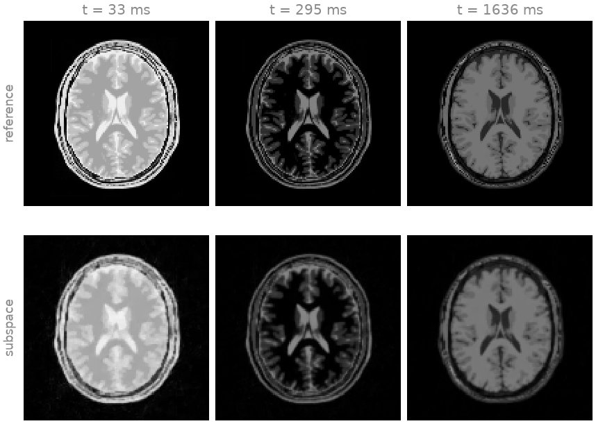
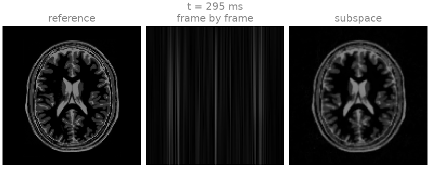
The three frames are shortly after the inversion, when every tissue is inverted and bright in magnitude; at the null of white matter, which is dark; and at the end of the train, in the steady state. The subspace reconstruction reproduces these contrast changes, each frame from its single spoke. The same frame reconstructed on its own is the streak pattern of one spoke, with no anatomy left in it.

The curve of a single voxel shows the same with its sign. The complex signal is rotated so that its steady state is positive and real. Because you normalized the data before the solve, the reconstruction determines the series only up to a global complex scale, so it is scaled to the reference in the least-squares sense.

The \(T_1\) map

The maps are drawn with the lipari colormap [6], in a window that spans white and grey matter; cerebrospinal fluid, beyond it, saturates. The difference maps are relative to the reference \(T_1\).

• 
• 

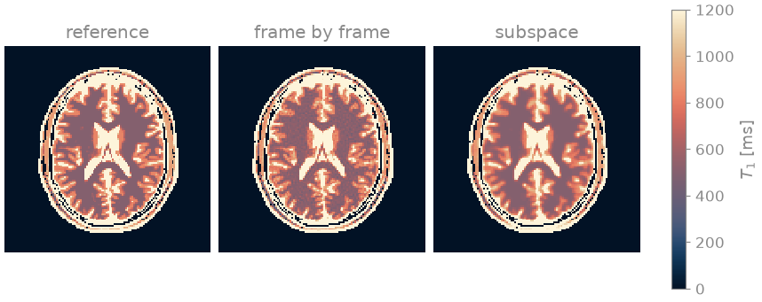
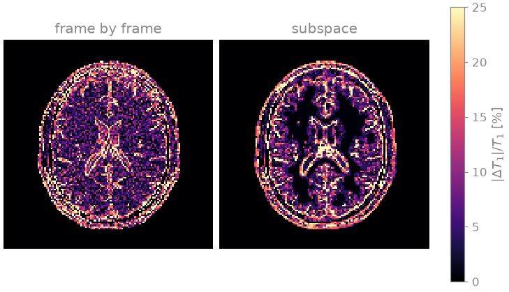
Matching the frames reconstructed one at a time still gives you a \(T_1\) map. The aliasing of each frame differs from that of the next, so along the recovery curve it is incoherent, and the match to the dictionary rejects much of it, which is the principle of MR fingerprinting [4]. What it does not reject stays as a voxel-to-voxel scatter over the whole head, which you see in the white matter of the difference map and in its standard deviation in the table. The subspace reconstruction fits the coefficient maps to all spokes at once under the total-variation penalty, and inside each tissue its error is a fraction of that of the frame-by-frame match.

Cerebrospinal fluid is the tissue the frame-by-frame match underestimates most. Its \(T_1\) is poorly determined by this acquisition: the recovery you observe during a gradient-echo train is governed by the apparent relaxation time \(T_1^* = (1/T_1 - \ln\cos\alpha / T_R)^{-1}\) [5], which for a flip angle \(\alpha\) of 6 degrees and a \(T_R\) of 4.1 ms is below 750 ms for any \(T_1\). The curves of long \(T_1\) therefore differ little from one another, and noise moves the match along the dictionary; a smaller flip angle or a longer train makes the acquisition more sensitive to long \(T_1\).

What both difference maps share is the rim of every tissue. A voxel holding two tissues follows the sum of two recovery curves, which is not itself a recovery curve, and the dictionary entry that matches it best has a \(T_1\) between the two. This partial-volume bias belongs to any voxelwise fit, not to the subspace, and it is why the whole-head error is larger than the interior one for both. The scalp fat is a layer one to two voxels thick, with no interior at this resolution, and is fitted between its own \(T_1\) and that of its neighbours.

As a spec

What this tour built, stated the way you would ask an agent for it:

Estimate a T1 map from one inversion-recovery spoiled gradient-echo
train of 400 shots (TR 4.1 ms, flip 6 degrees), one golden-angle radial
spoke per shot, 128 x 128, 8 coils, with bartorch. Simulate a
dictionary over 200 T1 values from 100 to 4500 ms with blochsim's
MPnRAGESimulator, and take its first 4 left singular vectors as the
basis. Build linop.NoncartesianSense over (4, y, x) with
traj (frames, 1, readout, 3) and basis=basis. Reconstruct the
coefficient maps with optim.ADMM (40 iterations, rho 0.05) and
priors.TotalVariation over the spatial axes, weight 0.001, on data
divided by optim.data_scaling. Match each voxel's coefficients to the
dictionary projected onto the basis by the normalized inner product,
and compare with matching frames gridded one at a time.

References

[1]

Tamir JI, Uecker M, Chen W, Lai P, Alley MT, Vasanawala SS, Lustig M. T2 shuffling: sharp, multicontrast, volumetric fast spin-echo imaging. Magn Reson Med 77(1):180-195 (2017). https://doi.org/10.1002/mrm.26102

[2]

Rudin LI, Osher S, Fatemi E. Nonlinear total variation based noise removal algorithms. Physica D 60(1-4):259-268 (1992). https://doi.org/10.1016/0167-2789(92)90242-F

[3]

Zhang T, Pauly JM, Levesque IR. Accelerating parameter mapping with a locally low rank constraint. Magn Reson Med 73(2):655-661 (2015). https://doi.org/10.1002/mrm.25161

[4]

Ma D, Gulani V, Seiberlich N, Liu K, Sunshine JL, Duerk JL, Griswold MA. Magnetic resonance fingerprinting. Nature 495(7440):187-192 (2013). https://doi.org/10.1038/nature11971

[5]

Deichmann R, Haase A. Quantification of T1 values by SNAPSHOT-FLASH NMR imaging. J Magn Reson 96(3):608-612 (1992). https://doi.org/10.1016/0022-2364(92)90347-A

[6]

Fuderer M, Wichtmann B, Crameri F, de Souza NM, Baeßler B, Gulani V, et al. Color-map recommendation for MR relaxometry maps. Magn Reson Med 93(2):490-506 (2025). https://doi.org/10.1002/mrm.30290

[7]

Collins DL, Zijdenbos AP, Kollokian V, Sled JG, Kabani NJ, Holmes CJ, Evans AC. Design and construction of a realistic digital brain phantom. IEEE Trans Med Imaging 17(3):463-468 (1998). https://doi.org/10.1109/42.712135