4. Joint reconstruction of image and sensitivity maps

In lesson 3 you saw ESPIRiT fail with eight ACS lines while nonlinear inversion kept working, because it fits the sensitivities to every acquired sample rather than to the ACS block alone. In this lesson you keep only six central lines, too few for any separate calibration, and reconstruct the image and the sensitivities together.

In the SENSE model

\[y_c = P F (S_c \cdot x)\]

both \(S_c\) and \(x\) become unknowns, and the model becomes bilinear: the data are a product of the two. Nonlinear inversion (NLINV) [2] solves it with the iteratively regularized Gauss-Newton method (IRGNM) [3]. The factorization into image and sensitivities is not unique, and NLINV restricts it by building smoothness of the sensitivities into the model. You first run it as BART’s nlinv, then write the same reconstruction out as an operator and a solver you can change.

Learning objectives

• Reconstruct an image and its sensitivities jointly with bartorch.tools.nlinv() from an ACS region too small for ESPIRiT.

• Explain the ambiguity of the bilinear model and how the Sobolev weighting of the sensitivities resolves it.

• Write the same reconstruction as bartorch.nlop.NonlinearSense under bartorch.nlop.IRGNM.

• See how the number of Gauss-Newton steps acts as a regularization parameter.

Previous: 3. Coil sensitivities. Next: 5. Choosing a regularizer, where you add a prior on the image to the reconstruction and learn how to choose it.

Simulated acquisition

The object is the BrainWeb slice of lesson 2 [1], at 128 by 128, and you receive it with BART’s analytical eight-channel head coil, as there. You keep a third of the phase encodes, drawn at random and more densely near the centre, but only six fully sampled lines at the centre itself. How the phantom and the pattern are made is hidden; lines is a vector of ones on the acquired phase encodes.

import torch

import bartorch
import bartorch.tools as bt

from bartorch import nlop

COILS = 8
ACCELERATION = 3
CALIBRATION = 6  # lines at the centre, far fewer than ESPIRiT needs

sensitivities = bt.coils(t=bt.grid(D=(SIZE, SIZE, 1)), n=COILS)[:, 0]
sensitivities /= bartorch.rss(sensitivities, axes=(0,), keepdim=True)

kspace = bartorch.fft(sensitivities * image, axes=(-2, -1), unitary=True)
kspace = bt.noise(kspace, n=1e-5, s=42)

lines = simulate(ACCELERATION, CALIBRATION)
pattern = lines.reshape(SIZE, 1).to(torch.complex64)
measured = kspace[:, None] * pattern

print(f"{float(lines.mean()):.0%} of the lines, {CALIBRATION} at the centre")

32% of the lines, 6 at the centre

Six central lines tell you where the centre of k-space is, but they do not calibrate anything on their own. ESPIRiT’s kernel is six points wide by default, so a six-line ACS region leaves it a single kernel position along the phase-encoding axis: far too few rows for the calibration matrix of bartorch.tools.ecalib().

Joint reconstruction

bartorch.tools.nlinv() takes the k-space and returns the image and, if you ask, the sensitivities it estimated on the way. maxiter counts Gauss-Newton steps, not linear iterations. The regularization weight is halved after every step, so the count is a regularization parameter rather than a convergence threshold: fewer steps give a smoother image, more steps admit more noise. BART’s default is eight steps; you use twelve.

STEPS = 12

reconstruction, estimated = bt.nlinv(
    measured,
    maxiter=STEPS,
    return_sensitivities=True,
)

channel_images = bartorch.ifft(measured[:, 0], axes=(-2, -1), unitary=True)
zero_filled = bartorch.rss(channel_images, axes=(0,))

for name, estimate in (("zero-filled", zero_filled), ("nlinv", reconstruction)):
    nrmse = bt.nrmse(image.abs(), estimate.abs(), scaled=True)
    print(f"NRMSE, {name:>11}: {nrmse:.3f}")

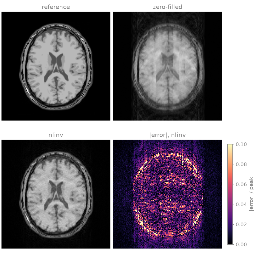
NRMSE, zero-filled: 0.209
NRMSE,       nlinv: 0.078

From a third of the phase encodes and six central lines, nonlinear inversion removes the aliasing of the zero-filled image. Its error sits at tissue boundaries, around the skull, and in the noise-like residue that random sampling leaves. As in lesson 2, scaled=True fits one global factor before comparing, so the NRMSE compares shapes, not the overall scale.

The estimated sensitivities

The coil unknown in NLINV is not the sensitivity map itself but its k-space representation \(\hat{s}\), and the map follows as

\[S = \mathcal{F}^{-1}\left[(1 + a|k|^2)^{-b/2} \, \hat{s}\right],\]

a Sobolev-norm weighting that suppresses high spatial frequencies. Every Gauss-Newton step in \(\hat{s}\) is therefore a smooth change of the map, and the joint problem needs no separate penalty on the coils.

This matters because the pair is determined only up to a common factor: multiply every map by a nonzero function \(\gamma(r)\), divide the image by it, and the data do not change (Model-based reconstruction). The weighting restricts \(\gamma\) to smooth functions, so your estimate can differ from the true maps by a smooth common magnitude and phase. To compare the two, you remove that factor: divide the maps by their root sum of squares and subtract the phase of channel 0.

maps = estimated[:, 0]
maps = maps / bartorch.rss(maps, axes=(0,), keepdim=True)
maps = maps * torch.exp(-1j * maps[0].angle())

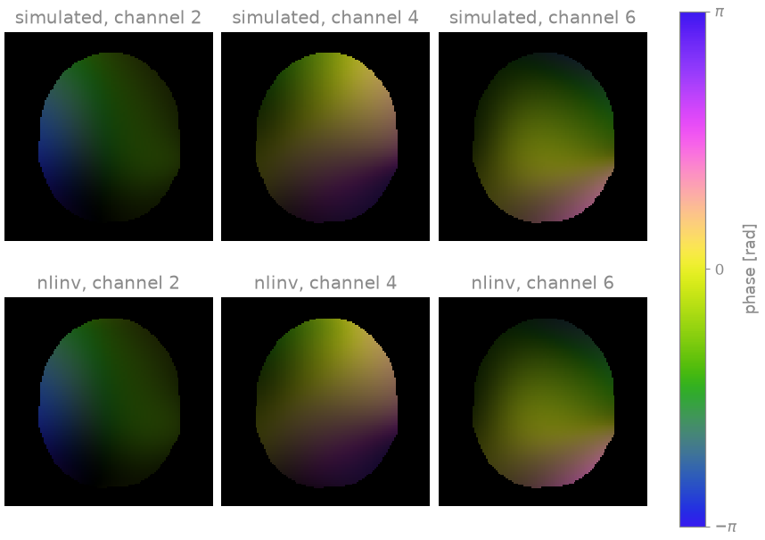
Inside the head, the normalized estimates reproduce the simulated maps in both magnitude and phase. Outside it neither factor is determined at all, since their product is zero there for any pair, so the maps follow from the initialization and the weighting; the figure masks them. nlinv reports its image multiplied by the root sum of squares of its maps, so the image it returns is the one that goes with maps normalized this way.

The model and the solver

nlinv runs a fixed configuration. To change any part of it, you write the model and the solver out explicitly. bartorch.nlop.NonlinearSense is the forward model above as a nonlinear operator with two inputs, the image and the coil coefficients, and bartorch.nlop.IRGNM is the Gauss-Newton loop over it. Each step linearizes the model at the current estimate \(x_k\) and solves

\[\min_x \, \| DF_{x_k} (x - x_k) - (y - F(x_k)) \|^2 + \alpha_k \| x - x_{\mathrm{ref}} \|^2,\]

where \(DF_{x_k}\) is the derivative of the forward model, \(x_{\mathrm{ref}}\) is zero unless you give one, and \(\alpha_k\) is halved after every step: the first steps are heavily regularized and the later ones are not.

model = nlop.NonlinearSense(
    (COILS, 1, SIZE, SIZE),
    pattern=lines.reshape(1, SIZE, 1).to(torch.complex64),
)
print(f"inputs {model.ishapes} -> output {model.oshapes}")

inputs ((1, 1, 128, 128), (8, 1, 128, 128)) -> output ((8, 1, 128, 128),)

To get what nlinv gets, you need three of its settings. It scales the data by \(100 / \|y\|\) before it starts, which fixes what \(\alpha\) means, and it runs the conjugate gradients of each step to a hundred iterations or a relative tolerance of a tenth:

scale = 100.0 / float(torch.linalg.vector_norm(measured))
data = model.prepare(measured * scale)

solver = nlop.IRGNM(iterations=STEPS, cg_maxiter=100, cg_tol=0.1)
fitted, coefficients = solver(data, model)

coil_maps = model.coils(coefficients)
combined = fitted.squeeze() * bartorch.rss(coil_maps[:, 0], axes=(0,))

largest difference from nlinv: 1.0e-03
NRMSE 0.078

The loop you wrote and the application agree to about a thousandth of the image peak, and give the same NRMSE, rather than agreeing to the last bit: the data scaling is computed here and inside the application by different expressions.

What the operator form gives you is access to everything around the step. You can hand the linearized problem to a solver from bartorch.optim instead of the conjugate gradients inside the library (inner=optim.CG() is the same method written out, and a regularized solver makes the step a regularized one), unroll the loop as bartorch.nlop.IRGNMBlock, and differentiate a Gauss-Newton step with respect to the data, the iterate, the regularization centre and \(\alpha\) (Learned reconstruction). Putting a signal model in front of the same encoding, to reconstruct parameter maps rather than an image, is lesson 9 (9. Nonlinear inversion for T2 mapping).

Exercise: Gauss-Newton steps

The number of Gauss-Newton steps was described above as a regularization parameter. Run nlinv for a few more step counts and compute the NRMSE of each image; the plot adds the twelve-step result from above:

counts = (4, 8, 16)
scores = []
for count in counts:
    estimate = bt.nlinv(measured, maxiter=count)
    scores.append(bt.nrmse(image.abs(), estimate.abs(), scaled=True))

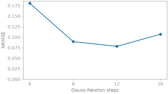
 4 steps: NRMSE 0.181
 8 steps: NRMSE 0.089
12 steps: NRMSE 0.078
16 steps: NRMSE 0.107

The error is lowest at twelve steps and higher on both sides. With four steps the regularization weight is still large and the estimate is biased towards the regularization centre; at sixteen the weight has been halved four more times and the noise amplified by the inversion dominates. The optimum depends on the noise level and the undersampling: try a different n in bt.noise and see where the minimum moves. Later steps are also more expensive than early ones, so a large step count costs considerably more time.

As a spec

What this lesson built, stated the way you would ask an agent for it:

With bartorch, reconstruct a 2D Cartesian 8-channel k-space of shape
(coils, 1, y, x), undersampled along y to a third of the lines with only
6 fully sampled central lines, by nonlinear inversion: bt.nlinv with 12
Gauss-Newton steps, returning the sensitivities. Then write the same
reconstruction as nlop.NonlinearSense (with the sampling pattern) under
nlop.IRGNM(iterations=12, cg_maxiter=100, cg_tol=0.1), on data scaled
by 100 / ||y||, and check it against bt.nlinv(normalize=False). Compare
the estimated maps with the true ones after dividing by their root sum
of squares and removing the phase of channel 0.

References

[1]

Collins DL, Zijdenbos AP, Kollokian V, Sled JG, Kabani NJ, Holmes CJ, Evans AC. Design and construction of a realistic digital brain phantom. IEEE Trans Med Imaging 17(3):463-468 (1998). https://doi.org/10.1109/42.712135

[2]

Uecker M, Hohage T, Block KT, Frahm J. Image reconstruction by regularized nonlinear inversion – joint estimation of coil sensitivities and image content. Magn Reson Med 60(3):674-682 (2008). https://doi.org/10.1002/mrm.21691

[3]

Bakushinsky AB, Kokurin MY. Iterative Methods for Approximate Solution of Inverse Problems. Springer (2004). https://doi.org/10.1007/978-1-4020-3122-9