

nlop.NonlinearSense#
- class bartorch.nlop.NonlinearSense#
Bases:
NonlinearOperatorJoint image and coil-sensitivity forward model, BART’s
noir.Two inputs, the image and the coil coefficients, and one output. The coil input is not the sensitivity maps but a k-space representation \(\hat{s}\) of them, mapped to the maps by the Sobolev weighting
\[S = \mathcal{F}^{-1} \left[ \, c \, (1 + a |k|^2)^{-b/2} \, \hat{s} \, \right]\](BART’s
noir_calc_weights), so the coils are smooth by construction and a Gauss-Newton step needs no separate penalty on them.coilsmaps fitted coefficients to sensitivities.On a grid the output is k-space. Off the grid, as BART builds the model, the output is the gridded coil images,
nufft^Hof k-space;prepare()brings a measurement to that form.- Parameters:
image_shape (tuple of int) – Coil-image shape
(coils, *spatial), C order, as the linear encodings take it. The image input is this shape with one coil.pattern (torch.Tensor, default=None) – Sampling mask on the grid, one at acquired positions;
Noneon a grid is all ones. Off the grid it is passed to BART as is and may not be combined withbasis.trajectory (torch.Tensor, default=None) – Trajectory
(..., samples, 3)in grid units, asbartorch.tools.traj()produces; selects the non-Cartesian model.kspace_shape (tuple of int, default=None) – Sample shape. Default:
image_shapeon a grid,(coils, *trajectory.shape[:-1], 1)off it.coil_shape (tuple of int, default=None) – Shapes of the sensitivities and of their coefficients; both default to
image_shape.coefficient_shape (tuple of int, default=None) – Shapes of the sensitivities and of their coefficients; both default to
image_shape.weights (torch.Tensor, default=None) – k-space diagonal applied to the samples off the grid; its conjugate is applied in the adjoint.
basis (torch.Tensor, default=None) – Temporal subspace basis
(coefficients, frames)over the last encoding axis; off the grid only.mask (torch.Tensor, default=None) – Support the image is restricted to.
sobolev (tuple of float, default=(220.0, 32.0)) –
(a, b)of the coil weighting; BART’s defaults.c (float, default=1.0) – Scale of the coil weighting.
real (bool, default=False) – Constrain the image to be real.
sos (bool, default=False) – BART’s sum-of-squares variant of the coil weighting.
oversampling_coils (float, default=None) – Grid oversampling of the coil coefficients;
Nonetakesnlinv’s choice, 2 off the grid and 1 on it.oversampled_coils (bool, default=False) – Return the sensitivities on the oversampled grid rather than the image’s.
toeplitz (bool, default=True) – Off the grid, apply the normal operator as a convolution with a point spread function rather than as a NUFFT and its adjoint.
optimized (bool, default=False) – Off the grid, BART’s
noir2_noncart_optimized_create.
- Raises:
ValueError – If
basisis given on a grid, or withpatternoff the grid.
Examples
>>> F = NonlinearSense((8, 128, 128), pattern=mask)
>>> F.ishapes
((1, 128, 128), (8, 128, 128))
>>> image, coefficients = nlop.IRGNM()(kspace, F)
- property coils#
Linear operator from coil coefficients to sensitivity maps.
The Sobolev weighting followed by the inverse Fourier transform.
- property image#
support mask and real constraint.
- Type:
Linear operator applied to the image input
- property data#
Linear operator from the model’s output to k-space.
The NUFFT off the grid, whose adjoint is
prepare(); the identity on a grid.
- property transform#
Linear operator from coil images to k-space, the encoding after the product.
- prepare()#
Bring a measurement to the model’s output.
Off the grid this is
nufft^H(kspace), asnoir2_reconapplies it before the first Gauss-Newton step; on a gridkspaceis returned unchanged.- Parameters:
kspace (torch.Tensor) – Measurement of
kspace_shape.- Returns:
Tensor of
oshape.- Return type:
torch.Tensor
Also has the methods and properties of NonlinearOperator.
Examples using NonlinearSense#
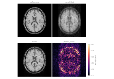
4. Joint reconstruction of image and sensitivity maps