Receive bias field

When you combine the images of a receive array by root sum of squares, what you get is the object weighted by the root sum of squares of the coil sensitivities. That weight is smooth, multiplicative and largest near the elements, so it shades the image: the same tissue looks brighter near the array than far from it. The shading biases segmentation, intensity-based registration and any quantitative comparison across the field of view.

In this tour you shade a T1-weighted head with a head array that has no anterior elements, estimate the field with N4 [1] through bartorch.tools.bias_field_correct(), and compare the corrected image and the estimated field with the object and the true field.

Prerequisites: lesson 1, 1. Your data as tensors.

Learning objectives

• Relate the shading of a root-sum-of-squares image to the receive sensitivities.

• Estimate and remove the bias field with N4, and judge the result by the uniformity of a tissue class and by the intensity histogram.

• Choose the mask and the fitting grid of the estimate.

• Recognise what N4 does not recover: the scale of the field, the steep part of a field of large range, and a smooth intensity variation that belongs to the object.

import torch

import bartorch
import bartorch.tools as bt

The object

Your object is an axial slice of the BrainWeb T1-weighted head [2] through the lateral ventricles, 128 x 128 over a 220 mm field of view. The BrainWeb tissue model also tells you which voxels are at least 90 % white or grey matter, and you measure the uniformity of each class over those.

SIZE, FOV_MM = 128, 220.0

The shaded image

The array is BART’s analytical eight-element head coil with its two anterior elements removed, as in an open-face head coil: six elements. Each coil image is the object weighted by one element’s sensitivity \(S_c\), plus independent complex Gaussian noise. Their root sum of squares is the object weighted by the bias field \(B = \sqrt{\sum_c |S_c|^2}\), and the noise adds a Rician floor in the background.

def shaded_image(elements):
    grid = bt.grid(D=(SIZE, SIZE, 1))
    sensitivities = bt.coils(t=grid, n=8)[elements, 0]
    bias = bartorch.rss(sensitivities, axes=(0,)).abs()
    sensitivities = sensitivities / bias[brain].mean()
    coil_images = bt.noise(sensitivities * image, n=1e-4, s=3)
    shaded = bartorch.rss(coil_images, axes=(0,)).abs()
    return shaded, bias / bias[brain].mean()


shaded, bias = shaded_image([0, 1, 2, 5, 6, 7])

bias field over the brain: 0.56 to 1.27 (2nd to 98th percentile)

N4 correction

N4 works on the logarithm of the image, where the field is no longer a factor but an additive term: the log of the object plus a smooth field, represented by cubic B-splines. It estimates the field by alternately sharpening the histogram of the log intensities and fitting the splines to what the sharpening removed, over a hierarchy of control-point grids. It knows nothing about the coil; all it needs is an object whose intensities form classes.

The field is fitted on the image shrunk by shrink_factor. The default of 4 would leave a 32 x 32 grid of this 128 matrix, so you pass 2, which keeps 64 x 64. Ask for the field as well as the corrected image:

corrected, estimate = bt.bias_field_correct(
    shaded,
    shrink_factor=2,
    return_field=True,
)

You measure the uniformity of a tissue class by its coefficient of variation, the standard deviation over the mean. The object has some too, from partial volume at the class boundaries, so that is the floor to compare with.

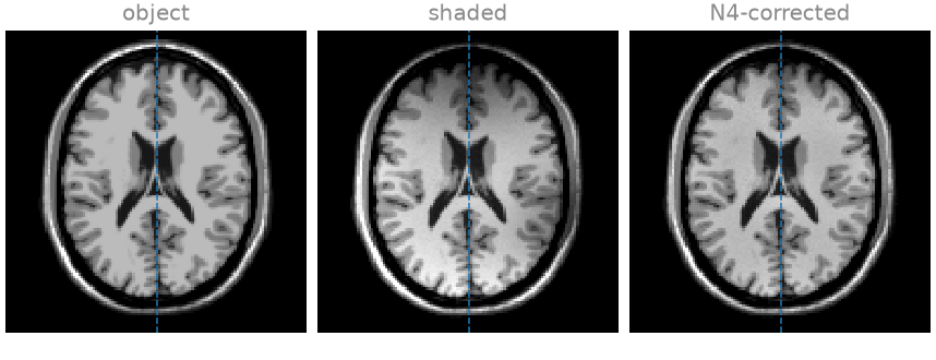
object        coefficient of variation: white matter 0.011, grey matter 0.035; white/grey 1.35
shaded        coefficient of variation: white matter 0.135, grey matter 0.193; white/grey 1.38
N4-corrected  coefficient of variation: white matter 0.035, grey matter 0.073; white/grey 1.35

The correction takes the white-matter variation from more than ten times the object’s to about three times it, and keeps the white/grey contrast of the object.

A multiplicative field is only determined up to a constant factor, and the correction leaves that factor in the image. So you compare the estimate with the true field after scaling both to unit mean over the brain:

estimate = estimate / estimate[brain].mean()

• 
• 
• 
• 

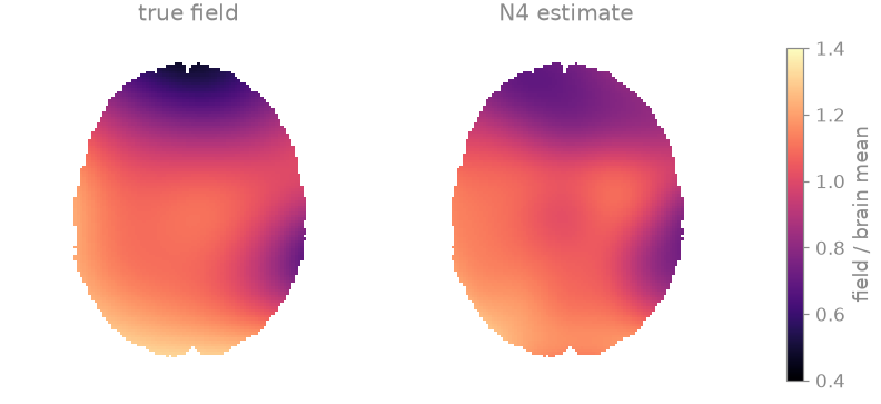
estimated / true field over the brain: median 0.997, within 10 % in 93 % of the voxels

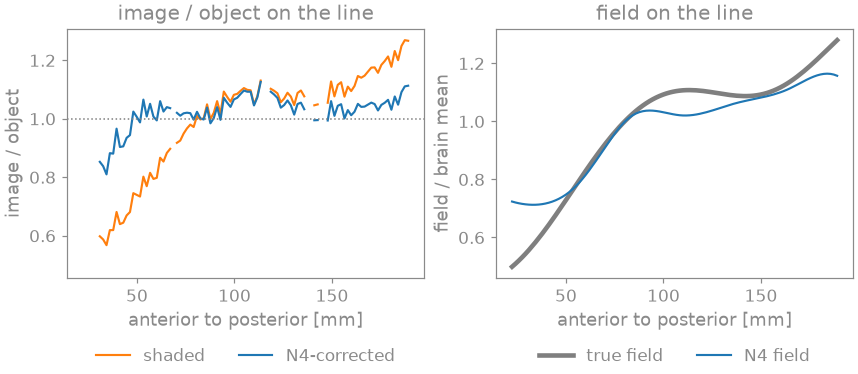
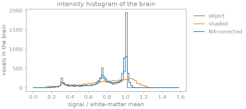
The images share one window, each scaled to its white-matter mean. In the shaded image you see the frontal lobes darker than the occipital lobes. Along the dashed line the ratio of the shaded image to the object follows the field, and the histogram of the brain has no separate grey- and white-matter peaks. After correction the ratio stays close to one except at the frontal pole, where the estimated field does not fall as far as the true one, and the two peaks separate again. Over the brain the estimated field is within 10 % of the true one in more than nine voxels out of ten.

The mask

N4 fits the field only over a mask, by default Otsu’s threshold of the image. You can give it a mask of the whole head instead, which adds the scalp and the skull, or a brain mask such as a skull-stripping tool gives you; here the BrainWeb tissue model provides it.

masks = {"Otsu": None, "head": torch.as_tensor(head), "brain": brain}
for name, mask in masks.items():
    trial = bt.bias_field_correct(shaded, mask=mask, shrink_factor=2)
    spread = variation(trial, white)
    print(f"{name:5s} mask: white-matter variation {spread:.3f}")

Otsu  mask: white-matter variation 0.035
head  mask: white-matter variation 0.063
brain mask: white-matter variation 0.023

N4 sharpens one histogram over the whole mask. The scalp and the skull bring intensity classes of their own, so the fit over the head mask is the least uniform. The brain mask, which holds only the classes you judge the field by, gives the most uniform white matter.

Residual bias

The estimate gets worse as the range of the field grows. Keep only the four posterior elements, and the field falls steeply towards the frontal pole:

steep, steep_bias = shaded_image([0, 1, 6, 7])
steep_corrected, steep_estimate = bt.bias_field_correct(
    steep,
    shrink_factor=2,
    return_field=True,
)

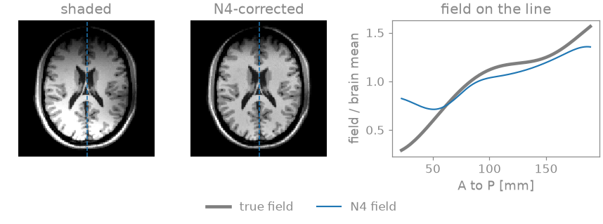
four posterior elements: field 0.35 to 1.55
white-matter variation: shaded 0.262, N4-corrected 0.096; estimate within 10 % in 83 % of the voxels

N4 overestimates the field at the frontal pole: its estimate does not fall as far as the true one, so the corrected frontal cortex stays darker than the occipital cortex. A residual like this is why you still compare a corrected image across regions with care.

There is a second limit, and it is not a failure of the fit. N4 removes any smooth intensity variation, whatever its origin: a receive field, a transmit field in a gradient-echo image, or a genuine slow change of the tissue signal. In a SENSE reconstruction the sensitivities are normalized to unit root sum of squares, which removes the receive shading inside the reconstruction. N4 is for images whose sensitivities you do not have, such as a root-sum-of-squares combination, and for the transmit field, which no receive calibration measures.

Exercise: B-spline fitting grid

The field is fitted on the shrunk image and evaluated on the full grid. A field that is smooth on the scale of the head needs few grid points, and each N4 iteration gets cheaper as their number falls. Vary shrink_factor and watch the white-matter uniformity:

for shrink in (1, 2, 4, 8):
    trial = bt.bias_field_correct(shaded, shrink_factor=shrink)
    spread = variation(trial, white)
    print(f"shrink_factor {shrink}: white-matter variation {spread:.3f}")

shrink_factor 1: white-matter variation 0.029
shrink_factor 2: white-matter variation 0.035
shrink_factor 4: white-matter variation 0.036
shrink_factor 8: white-matter variation 0.056

Factors of 1 to 4 do about equally well here. At 8 the shrunk image is 16 x 16 and holds too few voxels of each tissue class, and the variation rises.

As a spec

What this tour built, stated the way you would ask an agent for it:

Correct the receive bias field of a 2D root-sum-of-squares magnitude
image with bt.bias_field_correct (N4), shrink_factor 2, returning the
field. Compare a mask of None (Otsu), the whole head and the brain.
Report the coefficient of variation over white and grey matter before
and after, the white/grey contrast, and the fraction of brain voxels
where the estimated field, scaled to unit brain mean, is within 10 % of
the true field.

References

[1]

Tustison NJ, Avants BB, Cook PA, Zheng Y, Egan A, Yushkevich PA, Gee JC. N4ITK: improved N3 bias correction. IEEE Trans Med Imaging 29(6):1310-1320 (2010). https://doi.org/10.1109/TMI.2010.2046908

[2]

Collins DL, Zijdenbos AP, Kollokian V, Sled JG, Kabani NJ, Holmes CJ, Evans AC. Design and construction of a realistic digital brain phantom. IEEE Trans Med Imaging 17(3):463-468 (1998). https://doi.org/10.1109/42.712135