6. Custom encoding and solver

In lesson 5 you handed pics the data, the maps and a penalty, and it did the rest. In this lesson you assemble the same reconstruction from its parts. You build the SENSE encoding operator, check its adjoint, run the solver on it, and obtain exactly what pics returns, bit for bit. Then you extend the operator with one written in Python, and differentiate through it.

The mental model: bartorch.apps.pics() builds three objects and runs BART’s iteration on them: the encoding operator \(A = PFS\) (sensitivities, Fourier transform, sampling), the regularization terms of bartorch.priors, and an iterative algorithm of bartorch.optim. You need the parts whenever BART has no application for what you want to do: an encoding with an extra factor, such as an off-resonance or motion phase; a solver called from your own outer loop; an operator written in Python; or a gradient with respect to the data, to train a network.

Learning objectives

• Build bartorch.linop.CartesianSense and read the plan it was lowered into.

• Check an operator’s adjoint with the dot-product test.

• Prepare the data as pics does and reproduce bartorch.apps.pics() bit for bit with bartorch.optim.FISTA.

• Compose operators, include one defined in Python, and differentiate through an application.

Previous: 5. Choosing a regularizer. Next: 7. Basics of non-Cartesian imaging, where you replace the FFT with a NUFFT and leave the Cartesian grid.

The encoding operator

Your scan is the one of lesson 2 [1], with a tenth of its noise: eight channels, kspace of shape (coils, 1, y, x) with one phase-encoding line in three acquired around a 24-line ACS block. ESPIRiT gives you the maps, as before.

bartorch.linop.CartesianSense is \(A = PFS\) as one operator. You give it the sensitivities, the shape of the image, and the sampling pattern; the shape of the k-space it maps to follows from those. bartorch.tools.pattern() reads the pattern off the data, as you would for a prospectively undersampled scan.

modulated=True selects the uncentred sample convention that BART’s applications iterate in; the default is the centred convention of bartorch.fft(). The two differ by a modulation of the samples and give the same image. The choice matters only when you apply the operator to data already in one of them, as you do below.

import torch

import bartorch
import bartorch.tools as bt

from bartorch import apps, linop, optim, priors

maps = bt.ecalib(kspace, maps=1, calib_size=CALIBRATION, crop=0.8)
pattern = bt.pattern(kspace)

A = linop.CartesianSense(
    maps.squeeze(1),
    (SIZE, SIZE),
    pattern.squeeze(),
    modulated=True,
)
print(f"{A.ishape} -> {A.oshape}")
print(A.plan)
print(f"fused: {A.plan.fused}")

(192, 192) -> (8, 192, 192)
Plan(transform=fft, image=sensitivities, normal=transform, coil_batch=1, streamed=coils, executor=slab)
fused: True

The operator maps an image of (y, x) to k-space of (coils, y, x). A.plan reports how it is computed: which transform, what multiplies the image and the samples, and how the normal operator \(A^H A\) is applied. It is read back from the operator that was built, not predicted. plan.fused is false where the composition could not be expressed as one encoding and fell back to a chain, which gives the same numbers more slowly.

The adjoint

A solver needs \(A^H\), not \(A^T\), and one built on the wrong one converges to the wrong image. You can check it with the definition, \(\langle Ax, y\rangle = \langle x, A^H y\rangle\), which holds for any pair of vectors, random ones included:

generator = torch.Generator().manual_seed(0)
probe = torch.randn(A.ishape, dtype=torch.complex64, generator=generator)
samples = torch.randn(A.oshape, dtype=torch.complex64, generator=generator)

forward = (A(probe).conj() * samples).sum()
adjoint = (probe.conj() * A.H(samples)).sum()
print(f"relative difference {abs(forward - adjoint) / abs(forward):.2e}")

relative difference 1.20e-07

The two inner products agree to single-precision round-off.

Solving

A solver is called as solver(y, A). To get the answer pics gets, you give it the data pics iterates on rather than the array the scanner wrote: the sampling pattern applied, the modulation into the uncentred convention, and the data divided by the scale bartorch.optim.data_scaling() estimates.

measured = bartorch.fftmod(kspace * pattern, axes=(-1, -2, -3), inverse=True)
scale = optim.data_scaling(measured)
data = (measured / scale).squeeze(1)

term = priors.Wavelet(axes=(-1, -2), weight=0.002)
assembled = optim.FISTA(term, maxiter=100)(data, A) * scale

The solution is multiplied back by the scale, which puts the image into the units of the k-space, as pics does unless given rescale=False. Now run pics on the raw kspace with the same term and solver, and compare:

tool = apps.pics(kspace, maps, regularizers=term, solver="fista", maxiter=100)
same = torch.equal(assembled.squeeze(), tool.squeeze())
print(f"identical to pics: {same}")


def nrmse(estimate):
    return bt.nrmse(image.abs(), estimate.abs(), scaled=True)


print(f"NRMSE, adjoint {nrmse(A.H(data)):.3f}")
print(f"NRMSE, FISTA   {nrmse(assembled):.3f}")

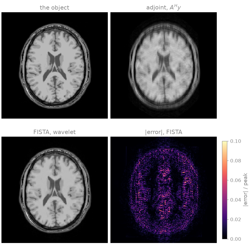
identical to pics: True
NRMSE, adjoint 0.119
NRMSE, FISTA   0.032

The two are the same iteration over the same operator, so they return the same bits, not merely close ones. In the figure, the adjoint \(A^H y\) is not the inverse: it is the sensitivity-weighted coil combination of the zero-filled k-space, and it carries the aliasing of the undersampling and the shading of \(\sum_c |S_c|^2\). The solve removes both, as the NRMSE printed above shows, and its remaining error sits at the tissue boundaries.

Operator algebra

@ composes, + adds, A.H is the adjoint and A.gram() the normal operator \(A^H A\). A composition builds one BART operator rather than a Python chain, so a solver iterating on it does not return to Python between applications. bartorch.optim.maxeigen() runs the power iteration on an operator; the largest eigenvalue of \(A^H A\) is the Lipschitz constant of the least-squares gradient, which bounds the gradient step size.

print(f"largest eigenvalue of A^H A: {optim.maxeigen(A.gram()):.3f}")

largest eigenvalue of A^H A: 0.999

An operator of your own is composed with BART’s operators through from_callbacks(): you give it the input and output shapes, a forward and an adjoint, and BART calls them back. Here it is a spatially varying phase, as an off-resonance or eddy-current phase would be, placed between the image and the encoding:

field = torch.exp(1j * 0.4 * torch.pi * grid_x).to(torch.complex64)
phase = linop.LinearOperator.from_callbacks(
    (SIZE, SIZE),
    (SIZE, SIZE),
    lambda u: field * u,
    lambda u: field.conj() * u,
)
composed = A @ phase
print(f"{composed.ishape} -> {composed.oshape}, fused: {composed.plan.fused}")

(192, 192) -> (8, 192, 192), fused: True

composed has the same interface as A (forward, adjoint, normal operator) and is passed to a solver in the same way.

Differentiation

Apply an operator to a tensor that requires a gradient, and autograd records it. For \(y = Ax\) the gradient torch propagates back is \(A^H g\), not \(A^T g\), which is torch’s conjugate Wirtinger convention for complex tensors. A real \(A\) has \(A^H = A^T\), so only a complex check tells the two apart. Here the gradient of \(\|Ax - y\|^2\) at \(x = 0\) should be \(-2A^H y\):

variable = data.new_zeros(A.ishape).requires_grad_(True)
residual = A(variable) - data
(residual.abs() ** 2).sum().backward()

expected = 2 * A.H(-data)
difference = (variable.grad - expected).abs().max() / expected.abs().max()
print(f"relative difference from 2 A^H (Ax - y): {float(difference):.2e}")

relative difference from 2 A^H (Ax - y): 2.06e-07

Learned reconstruction describes the backward passes of the solvers, and Solvers which algorithm applies to which problem.

Exercise: FISTA convergence

optim.FISTA is a loop over bartorch.optim.FISTABlock, one iteration per call. Run the loop yourself for 200 iterations and record the error of the image after each one:

block = optim.FISTABlock(term)
state = block.start(data, A)
trace = []
for _ in range(200):
    state = block(state, A)
    trace.append(nrmse(block.output(state, A)))

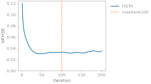
The error falls steeply over the first few tens of iterations, reaches its minimum before iteration 50, and then stays close to that level with small fluctuations up to iteration 200. For this data and weight, the 100 iterations used above are past the point where more iterations reduce the error. Try step=0.5 in FISTABlock, or a larger weight, and compare the curves.

As a spec

What this lesson built, stated the way you would ask an agent for it:

With bartorch, build linop.CartesianSense from ESPIRiT maps, the image
shape and the sampling pattern of a 2D Cartesian 8-channel k-space
(modulated=True), print its plan, and check its adjoint with a random
dot-product test. Prepare the data as pics does (pattern, fftmod
inverse, divided by optim.data_scaling), solve with optim.FISTA and
priors.Wavelet over the last two axes (weight 0.002, 100 iterations),
and check torch.equal against apps.pics with the same term. Compose the
operator with a Python phase operator from from_callbacks, and check
that autograd's gradient of ||Ax - y||^2 at zero is -2 A^H y.

References

[1]

Collins DL, Zijdenbos AP, Kollokian V, Sled JG, Kabani NJ, Holmes CJ, Evans AC. Design and construction of a realistic digital brain phantom. IEEE Trans Med Imaging 17(3):463-468 (1998). https://doi.org/10.1109/42.712135