Annealed plug-and-play

In lesson 10 you plugged a denoiser someone else had trained, on photographs, into ADMM at one noise level you chose. In this tour you train the denoiser yourself, on MR images alone and without any encoding, and use it as the regularizer of an ADMM reconstruction whose denoising strength decreases over the iterations. You then apply the same network, unchanged, at an acceleration where CG-SENSE breaks down.

A plug-and-play reconstruction [1] replaces the proximal step of an iterative algorithm by a denoiser. Because the denoiser is trained on images, not on k-space, one network serves every protocol whose images resemble its training images: a change of acceleration, sampling pattern or coil array needs no retraining. The proximal step of a regularizer \(\lambda\phi\) with ADMM penalty \(\rho\) is a Gaussian denoiser of noise variance \(\sigma^2 = \lambda/\rho\). The first iterates carry the strong incoherent aliasing of the undersampling and the last are nearly consistent with the data, so a noise level that decreases from one to the other [2] removes the aliasing first and preserves fine anatomy at the end. The penalty follows as \(\rho_k = \lambda/\sigma_k^2\), which keeps the balance between data consistency and denoising that \(\lambda\) sets.

Prerequisites: lesson 10, 10. Plug-and-play reconstruction, and lesson 11, 11. Training an unrolled network.

Learning objectives

• Train a denoiser conditioned on the noise level, noise=True in bartorch.learning.UNet, with bartorch.learning.Reconstruction.

• Give bartorch.priors.ImplicitPrior a schedule of noise levels and bartorch.optim.ADMMBlock the matching schedule of penalties.

• Compare an annealed schedule with a fixed noise level, iteration by iteration, and apply the same denoiser at a higher acceleration.

Data

You use the slices, coils and fourfold undersampling of Staged training of an unrolled network: BrainWeb [3] subject 0 to train the denoiser on, subject 4 to reconstruct. The acquisition is wrapped in a function, because you will change the acceleration at the end.

import lightning
import torch

import bartorch
import bartorch.tools as bt

from bartorch import learning, linop, optim, priors
from monai.metrics import PSNRMetric
from torch.utils.data import DataLoader

COILS = 8
ITERATIONS = 12
NOISE = 0.02

_ = torch.manual_seed(0)

train_images = brain_slices(subject=0, count=24)
valid_images = brain_slices(subject=4, count=8)

coils = bt.coils(t=bt.grid(D=(SIZE, SIZE, 1)), n=COILS)[:, 0]
sensitivities = coils / bartorch.rss(coils, axes=(0,), keepdim=True)


def acquisition(acceleration, seed):
    """Cartesian SENSE, one line in ``acceleration`` on average."""
    ky = torch.arange(SIZE) - SIZE / 2
    density = torch.exp(-0.5 * (ky / (SIZE / 6)) ** 2)
    chance = density / density.sum() * (SIZE / acceleration)
    draw = torch.rand(SIZE, generator=torch.Generator().manual_seed(seed))
    lines = draw < chance
    lines[SIZE // 2 - 4 : SIZE // 2 + 4] = True
    pattern = lines.to(torch.complex64)[:, None].expand(SIZE, SIZE)
    pattern = pattern.contiguous()
    return linop.CartesianSense(sensitivities, (SIZE, SIZE), pattern=pattern)


def measure(A, generator):
    made = []
    for x in valid_images:
        shape, kind = A.oshape, torch.complex64
        noise = torch.randn(shape, dtype=kind, generator=generator)
        made.append(A(x) + NOISE * noise)
    return made


A = acquisition(4, seed=1)
kspace = measure(A, torch.Generator().manual_seed(3))

Noise-conditioned denoiser

With noise=True the U-Net takes the noise level as an input and modulates its features with it, so one network covers a range of SNRs. You train it on pairs of a slice and the same slice with complex white Gaussian noise, at a standard deviation drawn log-uniformly between 0.5 and 20 per cent of the image’s peak for each pair (ComplexNet scales each image to unit peak). No coil sensitivities, sampling pattern or k-space enter the training.

LOW, HIGH = 0.005, 0.2

network = learning.UNet(2, spatial=2, widths=(16, 32, 64), noise=True)
denoiser = learning.ComplexNet(network, spatial=2)


def pairs(images):
    made = []
    for x in images:
        sigma = LOW * (HIGH / LOW) ** torch.rand(())
        noisy = x + sigma * torch.randn_like(x)
        made.append({"input": noisy, "target": x, "sigma": sigma.reshape(1)})
    return made


trainer = lightning.Trainer(
    max_epochs=30,
    accelerator="cpu",
    logger=False,
    enable_checkpointing=False,
    enable_model_summary=False,
    enable_progress_bar=False,
)
trainer.fit(
    learning.Reconstruction(denoiser, "denoiser", lr=2e-3),
    DataLoader(train_images, batch_size=4, shuffle=True, collate_fn=pairs),
    DataLoader(valid_images, batch_size=4, collate_fn=pairs),
)

/opt/hostedtoolcache/Python/3.12.15/x64/lib/python3.12/site-packages/lightning/pytorch/utilities/_pytree.py:21: `isinstance(treespec, LeafSpec)` is deprecated, use `isinstance(treespec, TreeSpec) and treespec.is_leaf()` instead.
/opt/hostedtoolcache/Python/3.12.15/x64/lib/python3.12/site-packages/lightning/pytorch/trainer/connectors/data_connector.py:434: The 'val_dataloader' does not have many workers which may be a bottleneck. Consider increasing the value of the `num_workers` argument` to `num_workers=3` in the `DataLoader` to improve performance.
/opt/hostedtoolcache/Python/3.12.15/x64/lib/python3.12/site-packages/lightning/pytorch/trainer/connectors/data_connector.py:434: The 'train_dataloader' does not have many workers which may be a bottleneck. Consider increasing the value of the `num_workers` argument` to `num_workers=3` in the `DataLoader` to improve performance.

You score every image by the mean PSNR of its magnitude over the eight slices of subject 4. First the denoiser on its own, at three noise levels:

psnr = PSNRMetric(max_val=1.0)
truth = torch.stack(valid_images).abs()[:, None]


def score(images):
    return float(psnr(images.abs()[:, None], truth).mean())


with torch.no_grad():
    for sigma in (0.01, 0.05, 0.1):
        noisy = torch.stack(valid_images)
        noisy = noisy + sigma * torch.randn_like(noisy)
        level = torch.tensor([sigma])
        denoised = torch.stack([denoiser(x[None], level)[0] for x in noisy])
        before, after = score(noisy), score(denoised)
        print(f"sigma {sigma}: {before:5.2f} dB noisy, {after:5.2f} denoised")

sigma 0.01: 41.46 dB noisy, 41.13 denoised
sigma 0.05: 27.17 dB noisy, 27.16 denoised
sigma 0.1: 21.06 dB noisy, 21.06 denoised

The gain grows with the noise level: about 2 dB at 0.01, about 8 dB at 0.1. One set of weights covers the whole range, which is what lets the noise level change from one iteration to the next below.

Annealing schedules

ImplicitPrior takes a sequence of noise levels, one per iteration, and ADMMBlock a sequence of penalties; the last value of each is repeated past its end. The annealed schedule decreases the noise level geometrically from 0.1 to 0.01 of the peak over twelve iterations, and the penalty follows as \(\rho_k = \lambda/\sigma_k^2\). When the penalty changes, the block rescales ADMM’s scaled dual variable by the ratio of the old penalty to the new, so the unscaled one carries over. The two fixed schedules hold the noise level at 0.03 and at 0.01, with the penalty given by the same \(\lambda\).

LAMBDA = 1e-4

schedules = {
    "annealed, 0.1 to 0.01": torch.logspace(-1.0, -2.0, ITERATIONS),
    "fixed, 0.03": torch.full((ITERATIONS,), 0.03),
    "fixed, 0.01": torch.full((ITERATIONS,), 0.01),
}


def plug_and_play(sigma, lam=LAMBDA):
    prior = priors.ImplicitPrior(denoiser, sigma=sigma.tolist())
    rho = (lam / sigma**2).tolist()
    block = optim.ADMMBlock(prior, rho=rho, cg_maxiter=5)
    return learning.Unrolled(block, iterations=ITERATIONS)

steps() yields every iterate, so you can follow each schedule iteration by iteration:

curves, results = {}, {}
with torch.no_grad():
    for name, sigma in schedules.items():
        runs = [list(plug_and_play(sigma).steps(y, A)) for y in kspace]
        iterates = [torch.stack(images) for images in zip(*runs)]
        curves[name] = [score(images) for images in iterates]
        results[name] = iterates[-1]
cg = torch.stack([optim.cg(y, A, maxiter=20) for y in kspace])
results["CG SENSE, 20 iterations"] = cg

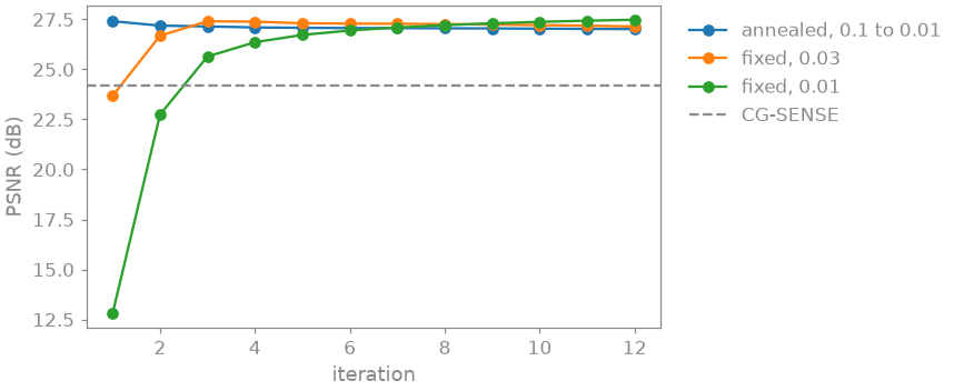
  annealed, 0.1 to 0.01   PSNR 27.01 dB
            fixed, 0.03   PSNR 27.14 dB
            fixed, 0.01   PSNR 27.48 dB
CG SENSE, 20 iterations   PSNR 24.21 dB

The fixed level of 0.03 converges within about four iterations, to an image limited by the smoothing the denoiser applies at that level. The fixed level of 0.01 preserves more detail, but its large penalty makes each ADMM step move little from the previous one: it starts far below CG-SENSE and is still rising after twelve iterations. The annealed schedule is ahead from the first iteration, and ends slightly ahead of the better fixed level, without a level having been tuned for this acquisition.

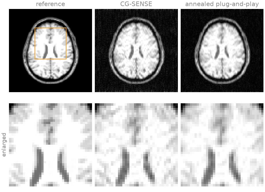
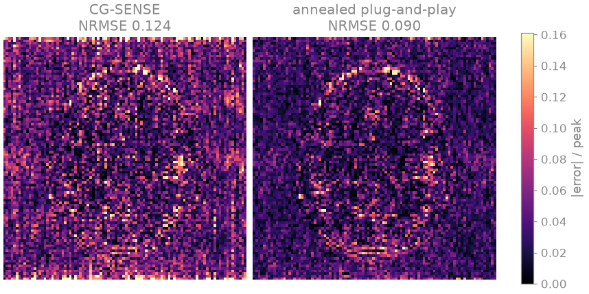
In the error maps of one slice, the CG-SENSE error is spread over the whole field of view; the plug-and-play error is confined to the head and largest at the cortex.

• 
• 

Transfer to another acquisition

You trained the denoiser without an encoding, so it applies unchanged to \(R = 6\), a sampling pattern it has never been used with:

A6 = acquisition(6, seed=2)
kspace6 = measure(A6, torch.Generator().manual_seed(4))
annealed_pnp = plug_and_play(schedules["annealed, 0.1 to 0.01"])
with torch.no_grad():
    annealed = torch.stack([annealed_pnp(y, A6) for y in kspace6])
cg6 = torch.stack([optim.cg(y, A6, maxiter=20) for y in kspace6])
print(f"R = 6: annealed plug-and-play {score(annealed):5.2f} dB")
print(f"R = 6: CG SENSE {score(cg6):5.2f} dB")

• 
• 

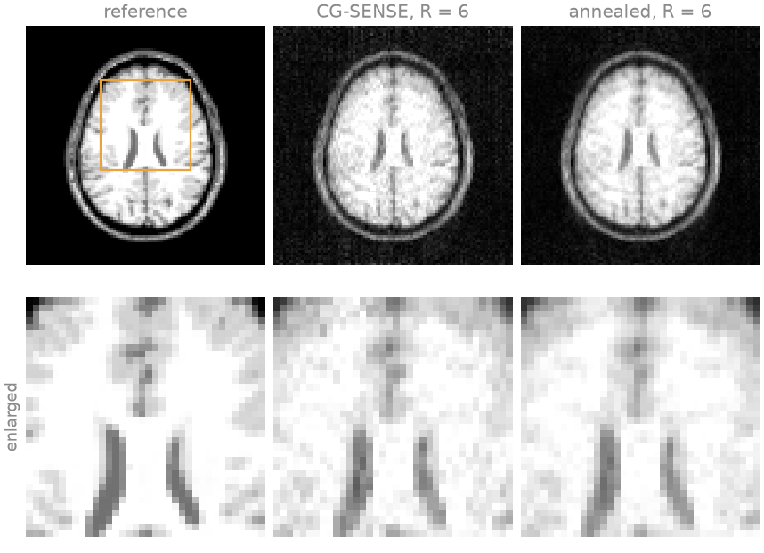
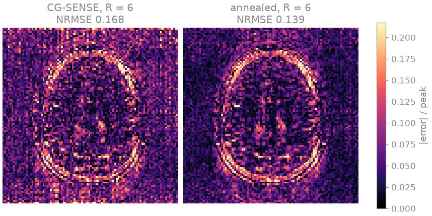
R = 6: annealed plug-and-play 23.72 dB
R = 6: CG SENSE 21.98 dB

At this acceleration eight coils no longer unfold the aliasing well: CG-SENSE loses about 2 dB with respect to \(R = 4\), and its error map shows the folded outline of the head on top of the g-factor noise. The plug-and-play reconstruction loses a fraction of a decibel and keeps the anatomy.

Exercise: the weight \(\lambda\)

\(\lambda\) sets the weight of the denoising step relative to data consistency at every noise level. Rerun the annealed schedule at \(R = 4\) with a tenth and ten times the weight above; the denoiser stays as it is:

for lam in (LAMBDA / 10, LAMBDA, LAMBDA * 10):
    pnp = plug_and_play(schedules["annealed, 0.1 to 0.01"], lam=lam)
    with torch.no_grad():
        made = torch.stack([pnp(y, A) for y in kspace])
    print(f"lambda {lam:.0e}: PSNR {score(made):5.2f} dB")

lambda 1e-05: PSNR 27.01 dB
lambda 1e-04: PSNR 27.01 dB
lambda 1e-03: PSNR 27.37 dB

Both a tenth and ten times the weight score more than 1 dB below \(\lambda = 10^{-4}\). A smaller \(\lambda\) lowers every penalty \(\rho_k\), so the denoiser’s output enters the data-consistency step with less weight; a larger one weights it more, and the reconstruction moves away from the measured data.

As a spec

What this tour built, stated the way you would ask an agent for it:

Train a noise-conditioned denoiser, ComplexNet(UNet(2, spatial=2,
widths=(16, 32, 64), noise=True)), on clean complex brain slices with
complex Gaussian noise of a log-uniform level in [0.005, 0.2], 30 epochs
of learning.Reconstruction(..., "denoiser", lr=2e-3). Use it as the
proximal step of 12 ADMM iterations (optim.ADMMBlock, 5 CG steps) for 2D
Cartesian SENSE at R = 4: priors.ImplicitPrior with sigma decreasing
geometrically from 0.1 to 0.01 and rho_k = 1e-4 / sigma_k^2. Compare it
with fixed sigma 0.03 and 0.01 and with CG-SENSE by PSNR per iteration,
and rerun it unchanged at R = 6.

References

[1]

Venkatakrishnan SV, Bouman CA, Wohlberg B. Plug-and-play priors for model based reconstruction. IEEE Global Conference on Signal and Information Processing 945-948 (2013). https://doi.org/10.1109/GlobalSIP.2013.6737048

[2]

Zhang K, Li Y, Zuo W, Zhang L, Van Gool L, Timofte R. Plug-and-play image restoration with deep denoiser prior. IEEE Trans Pattern Anal Mach Intell 44(10):6360-6376 (2022). https://doi.org/10.1109/TPAMI.2021.3088914

[3]

Collins DL, Zijdenbos AP, Kollokian V, Sled JG, Kabani NJ, Holmes CJ, Evans AC. Design and construction of a realistic digital brain phantom. IEEE Trans Med Imaging 17(3):463-468 (1998). https://doi.org/10.1109/42.712135