

Note
Go to the end to download the full example code.
EPI Nyquist ghost and ramp sampling#

An EPI readout acquires k-space as a train of lines with alternating readout gradient polarity, and before those lines make a Cartesian k-space you correct two things. A timing error between the readout gradient and the ADC, and eddy currents, shift the echoes of the reversed lines against the forward ones; the odd/even phase this leaves gives you a Nyquist ghost, a copy of the object shifted by half the field of view along the phase-encoding direction. And if you sample on the ramps of the readout gradient, to shorten the echo spacing, your samples are uniform in time but not in \(k_x\).
In this tour you simulate an eight-channel EPI acquisition of a Shepp-Logan phantom with a known ADC delay and constant phase error, estimate the odd/even phase from a three-line navigator, and remove the ghost. Then you resample a ramp-sampled readout onto a uniform \(k_x\) grid.
Prerequisites: lesson 1, 1. Your data as tensors.
Learning objectives
Relate an ADC delay to a linear phase in hybrid space, and that phase to the ghost at half the field of view.
Estimate the odd/even phase from a three-line navigator with
estimate_epi_phase(), and apply it to the reversed lines withcorrect_lines().Measure the ghost by its ghost-to-signal ratio.
Resample a ramp-sampled readout with
epi_ramp_operator(), and check the sampling condition under which that resampling is exact.
import math

import torch

import bartorch
import bartorch.tools as bt
The Nyquist ghost#
Here is the mental model. Say the ADC starts \(\delta\) dwell times late relative to the readout gradient. Every echo then moves by the same time: towards positive \(k_x\) on a forward line and towards negative \(k_x\) on a reversed one. In hybrid space, after the inverse Fourier transform along the readout, a shift of \(\delta\) dwell times is a linear phase \(\pi \delta u\) over the readout coordinate \(u \in [-1, 1]\). A constant phase \(\phi_0\), from eddy currents or a \(B_0\) offset during the readout, adds to it with the same alternating sign. So forward lines carry \(+(\pi \delta u + \phi_0)\) and reversed lines \(-(\pi \delta u + \phi_0)\). That difference between odd and even lines modulates k-space at the Nyquist frequency of the phase-encoding direction, and the image picks up a ghost at half the field of view.
You simulate it with a delay of a fifth of a dwell time and a constant phase of a quarter radian:
SIZE = 128
DELAY = 0.2  # dwell times
PHASE_0 = 0.25  # rad
SLOPE = math.pi * DELAY * (SIZE - 1) / SIZE  # rad over u in [-1, 1]

kspace = bt.phantom(SIZE, kspace=True, coils=8)[:, 0]  # (coils, ky, kx)
acquire(row, polarity) plays one line of the hybrid-space k-space with
the delay and the phase above, and returns it in the order the ADC
digitised it: a reversed line comes out flipped along the readout. Your EPI
train is a list of (line, reversed) pairs, which is the form
correct_lines() takes:
train = []
for ky in range(SIZE):
    reversed_line = ky % 2 == 1
    polarity = -1 if reversed_line else 1
    train.append((acquire(hybrid[:, ky], polarity), reversed_line))
The correction#
correct_lines() flips the reversed lines back into
readout order and, given the fit, removes the odd/even phase from them. That
brings them into phase with the forward lines. The phase the forward lines
keep is common to every line, so it does not change the magnitude image.
Without a fit it only flips:
ghosted_lines = bt.correct_lines(train)
corrected_lines = bt.correct_lines(train, fit)


def reconstruct(lines):
    stacked = torch.stack(lines, dim=1)  # (coils, ky, kx)
    coil_images = bartorch.ifft(stacked, axes=(-2, -1), unitary=True)
    return bartorch.rss(coil_images, axes=(0,)).abs()


ideal = reconstruct([kspace[:, ky] for ky in range(SIZE)])
ghosted = reconstruct(ghosted_lines)
corrected = reconstruct(corrected_lines)
You measure the ghost by the ghost-to-signal ratio: the mean signal outside the object divided by the mean signal inside it.
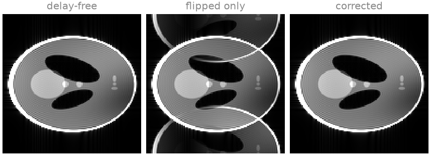
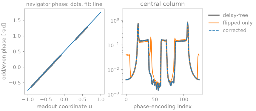
  delay-free: ghost-to-signal  1.38 %, NRMSE 0.0e+00
flipped only: ghost-to-signal 18.22 %, NRMSE 3.2e-01
   corrected: ghost-to-signal  1.38 %, NRMSE 1.1e-07
The images run from zero to 30 % of the peak, with phase encoding vertical. With the lines only flipped, you see the ghost at the top and bottom of the field of view, overlapping the object where it wraps. On the left, the navigator phase falls on a straight line, and the first-order fit goes through it. With that fit applied, the ghost-to-signal ratio is back to that of the delay-free image, whose signal outside the object is the truncation ringing of the phantom; in the central column the corrected profile lies on the delay-free one. It comes back exactly because the phase error you simulated is exactly first order. On measured data, higher orders of the phase, and phase errors that differ between lines of the same polarity, leave a residual ghost.
Ramp sampling#
If you sample on the ramps of the trapezoidal readout gradient, the samples
land at \(k_x(t) = \gamma \int_0^t G_x(\tau)\, d\tau\): denser on the
ramps than on the plateau. The readout is the Fourier transform of an object
that spans support pixels, so samples at any positions determine it, as
long as no two neighbouring samples are further apart than one over the
support, the Nyquist spacing of that object.
epi_ramp_operator() [1] is a matrix: the
regularized least-squares inverse of the transform at the sampled positions,
followed by the transform at the uniform ones.
Your readout gradient is a trapezoid whose ramps each take 30 % of the ADC window, sampled with 160 samples, and the object is one-dimensional, 64 pixels wide. Positions are in cycles per pixel.
SUPPORT, SAMPLES = 64, 160
RAMP = 0.3

time = torch.linspace(0.0, 1.0, SAMPLES, dtype=torch.float64)
gradient = torch.clamp(torch.minimum(time / RAMP, (1 - time) / RAMP), 0, 1)
sampled_at = torch.cumsum(gradient, 0)
sampled_at = sampled_at - sampled_at.mean()
sampled_at = 0.5 * sampled_at / sampled_at.abs().max()
uniform_at = torch.arange(SAMPLES, dtype=torch.float64) / SAMPLES - 0.5
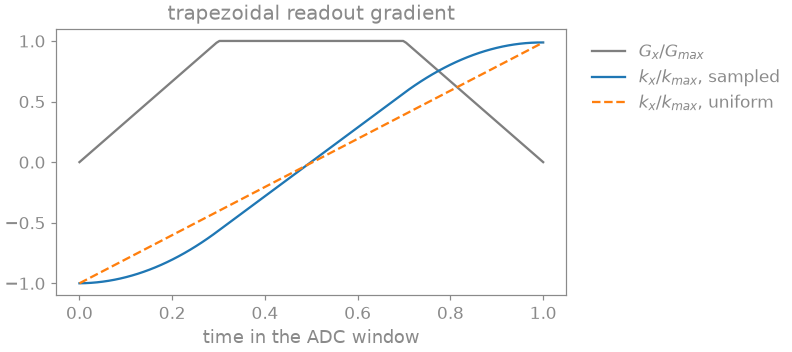
The sampled \(k_x\) curves on the ramps and is straight on the plateau, where it is steeper than the uniform grid you want to end on.
measured is the readout of a 64-pixel profile at the sampled positions
and truth the same readout on the uniform grid; how they are simulated
is hidden. You build the operator once from the trajectory and apply it to
every line of the train:
measured, truth = encode(sampled_at), encode(uniform_at)

operator = bt.epi_ramp_operator(sampled_at, uniform_at, SUPPORT)
resampled = measured.to(torch.complex64) @ operator.T
Linear interpolation between neighbouring samples is the comparison. You judge both on the image profile, the inverse transform of the uniform samples, and you check the sampling condition: the largest step between samples, times the support, has to stay below one.
step = float(torch.diff(sampled_at).max()) * SUPPORT
print(f"largest step x support: {step:.2f}")
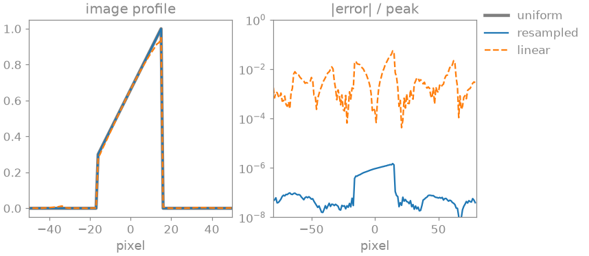
largest step x support: 0.57
 band-limited resampling: image NRMSE 1.4e-06
    linear interpolation: image NRMSE 3.2e-02
The step stays below one, so the resampling is exact up to the precision of the operator, which is returned in single precision: its error sits near \(10^{-6}\) of the peak and below. Linear interpolation errs most on the plateau, where the samples are furthest apart, and in the image its error spreads over the whole field of view, inside and outside the object, at up to a few per cent of the peak. On a measured trajectory the printed ratio is the thing to check: where a step exceeds one over the support, the readout is aliased and no resampling recovers it.
Exercise: readout delay#
Change the ADC delay, acquire the train and the navigator again, and compare the ghost-to-signal ratio with the lines only flipped and with the fit applied:
for delay in (0.1, 0.5, 1.0):
    SLOPE = math.pi * delay * (SIZE - 1) / SIZE
    lines = []
    for ky in range(SIZE):
        polarity = -1 if ky % 2 else 1
        lines.append((acquire(hybrid[:, ky], polarity), polarity < 0))
    navigator = [
        acquire(centre, 1),
        torch.flip(acquire(centre, -1), [-1]),
        acquire(centre, 1),
    ]
    fit = bt.estimate_epi_phase(navigator)
    before = ghost_to_signal(reconstruct(bt.correct_lines(lines)))
    after = ghost_to_signal(reconstruct(bt.correct_lines(lines, fit)))
    print(f"delay {delay:.1f}: {100 * before:5.2f} % -> {100 * after:5.2f} %")
delay 0.1: 11.61 % ->  1.38 %
delay 0.5: 47.86 % ->  1.38 %
delay 1.0: 51.12 % ->  1.38 %
The ghost grows with the delay, and the correction takes it back to the
delay-free level every time: the phase you simulate stays first order
whatever its slope, so the navigator fit describes it exactly. Try adding a
quadratic term to the phase in acquire and see what is left.
As a spec#
What this tour built, stated the way you would ask an agent for it:
Given an EPI train as a list of (line, reversed) pairs, each line a
(coils, readout) tensor in acquisition order, and a three-line
navigator (forward, reversed flipped into readout order, forward),
estimate the first-order odd/even phase with bt.estimate_epi_phase and
apply it with bt.correct_lines(train, fit). Report the ghost-to-signal
ratio before and after. For a ramp-sampled readout with known sample
positions in cycles per pixel, build bt.epi_ramp_operator(sampled,
uniform, support), apply it to every line, and check that the largest
sample step times the support is below 1.
References#
Total running time of the script: (0 minutes 2.838 seconds)