7. Basics of non-Cartesian imaging

In lessons 2 to 6 every sample sat on the Cartesian grid, so the FFT and its inverse were all the Fourier transforms you needed. In this lesson you leave the grid. You sample the same brain slice along radial and spiral trajectories, reconstruct it by gridding, and see what each step of that reconstruction does to the image.

The mental model: a radial or spiral readout starts at the centre of k-space and traces a curve through it, so its samples do not lie on a grid and the FFT cannot compute them. The non-uniform FFT (NUFFT) takes its place. Every non-Cartesian transform in bartorch is computed by FINUFFT [2], which evaluates

\[y_j = \frac{1}{\sqrt{N}} \sum_{m} x_m \, \exp\!\Big(-2\pi i \sum_d \frac{k_{j,d}\, m_d}{n_d}\Big)\]

to a requested tolerance. The sum runs over the \(N\) voxels \(m\) of an image with \(n_d\) voxels along dimension \(d\), and \(k_j\) is the position of sample \(j\) in grid units. Non-Cartesian transform states the conventions and the accuracy.

Learning objectives

• Generate radial and golden-angle trajectories in grid units with bartorch.tools.traj(), and a spiral trajectory by hand.

• Apply bartorch.nufft() and bartorch.nufft_adjoint(), and check the transform against the sum that defines it.

• Explain why a gridding reconstruction needs density compensation, and compute the weights analytically and with bartorch.estimate_density().

• Apply the normal operator \(A^H A\) as a convolution, and relate the point spread function (PSF) of an undersampled radial trajectory to its streaks.

Previous: 6. Custom encoding and solver. Next: 8. Radial SENSE, where you remove the streaks of an undersampled radial scan with the coils and a penalty.

Radial trajectory

The object is the BrainWeb slice of lesson 2 [1] on a 128 by 128 grid, acquired with a single receive coil of uniform sensitivity, so that the trajectory is the only encoding.

A trajectory in bartorch is a tensor of shape (*encoding, shots, samples, 3) holding the k-space position of every sample in grid units: one unit is one k-space cell of the image, so a readout of SIZE samples runs from \(-n/2\) to \(n/2\) for an image of \(n\) voxels. The last axis is \((k_x, k_y, k_z)\); \(k_z\) is zero throughout here, and that is what makes the transform two-dimensional.

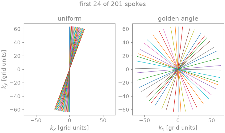
You can space the spokes of a radial scan in two ways. Uniformly, at \(\pi\) over their number, they tile k-space evenly once all of them are acquired. At the golden angle, every next spoke falls into the largest gap left by the previous ones, so any run of consecutive spokes tiles k-space nearly evenly [3]. That is what lets you cut a golden-angle scan into frames after you have acquired it, as the Tour Dynamic golden-angle radial MRI does.

import time

import torch

import bartorch
import bartorch.tools as bt

from bartorch import linop

SPOKES = 201  # pi/2 * SIZE: enough spokes not to undersample the edge

uniform = bt.traj(readout=SIZE, spokes=SPOKES, radial=True)
golden = bt.traj(readout=SIZE, spokes=SPOKES, radial=True, golden=True)
print(f"trajectory {tuple(golden.shape)}: (spokes, samples, 3)")

trajectory (201, 128, 3): (spokes, samples, 3)

You see the first 24 spokes of each scan. The uniform ones cover a narrow wedge, because they are spaced for 201 spokes and you would need all of them to fill the disc. The golden-angle ones already spread over every direction.

The transform

bartorch.nufft() samples an image along a trajectory, and bartorch.nufft_adjoint() takes samples back onto the grid. Since FINUFFT computes the transform only to a tolerance, check it once against the sum that defines it, evaluated by hand in double precision over the first spoke. That sum is computed without BART or FINUFFT, so it is an independent reference.

samples = bartorch.nufft(image, golden)
print(f"samples {tuple(samples.shape)}")

spoke = golden[0].real.double()  # (samples, 3)
m = torch.arange(SIZE, dtype=torch.float64) - SIZE // 2
my, mx = torch.meshgrid(m, m, indexing="ij")
km = spoke[:, :1] * mx.reshape(1, -1) + spoke[:, 1:2] * my.reshape(1, -1)
fourier = torch.exp(-2j * torch.pi / SIZE * km)
explicit = fourier @ image.reshape(-1, 1).to(torch.complex128) / SIZE

error = (explicit - samples[0]).abs().max() / explicit.abs().max()
print(f"largest relative difference from the sum: {float(error):.1e}")

samples (201, 128, 1)
largest relative difference from the sum: 1.9e-04

The difference sits within the tolerance the transform was planned with: a thousandth by default, on a grid a quarter larger than the image. That is meant for reconstruction, where the transform’s error stays small beside the noise and the undersampling; bartorch.linop.NUFFT takes oversampling and width when you need more accuracy.

Density compensation

The adjoint is not the inverse. Every spoke passes through the centre of k-space, so the sample density is highest there and decreases outwards: the sampling density of a radial scan falls as \(1/\lvert k \rvert\). The adjoint sums the samples unweighted, so it overweights the low frequencies. To undo that you weight each sample by the inverse of the sampling density [4], which for radial sampling is the ramp \(\lvert k \rvert\). The clamp keeps a small weight on the samples at the centre, which would otherwise not count at all.

def ramp(trajectory):
    """The radial density compensation, |k| per sample."""
    k = torch.linalg.norm(trajectory.real[..., :2], dim=-1, keepdim=True)
    return k.clamp(min=0.25).to(torch.complex64)


shape = (SIZE, SIZE)
plain = bartorch.nufft_adjoint(samples, golden, image_shape=shape)
compensated = bartorch.nufft_adjoint(
    samples * ramp(golden),
    golden,
    image_shape=shape,
)

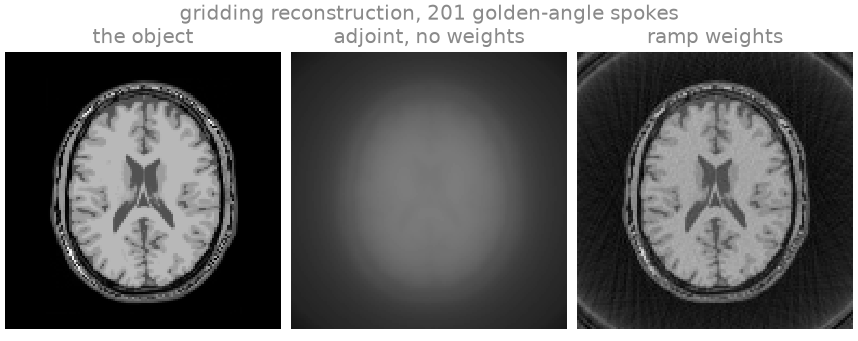
Without weights the image is blurred: it is the object convolved with the PSF of the trajectory, which is broad because the sample density is concentrated at the centre of k-space. With the ramp weights the tissue boundaries are resolved. Neither image recovers what the trajectory never reaches: a radial scan covers a disc, so the corners of the Cartesian k-space are missing whatever the weights are.

Estimated density

The ramp is the density of an ideal radial trajectory. For any other trajectory, bartorch.estimate_density() estimates the weights with the fixed-point iteration of Pipe and Menon [4], which runs on the same NUFFTs. It takes the coordinates as (..., samples, 2), so you flatten the spokes into one list of samples and reshape the weights back.

flat = golden.real[..., :2].reshape(-1, 2)
estimated = bartorch.estimate_density(flat, shape)
estimated = estimated.reshape(SPOKES, SIZE, 1).to(torch.complex64)

for name, density in (("ramp", ramp(golden)), ("Pipe-Menon", estimated)):
    weighted = samples * density
    adjoint = bartorch.nufft_adjoint(weighted, golden, image_shape=shape)
    nrmse = bt.nrmse(image.abs(), adjoint.abs(), scaled=True)
    print(f"{name:>10}  NRMSE {nrmse:.3f}")

      ramp  NRMSE 0.297
Pipe-Menon  NRMSE 0.278

For a radial trajectory the two weightings give similar errors, and both include the corners the disc does not cover. The estimate is needed where no closed form is available, as for a spiral.

Spiral trajectory

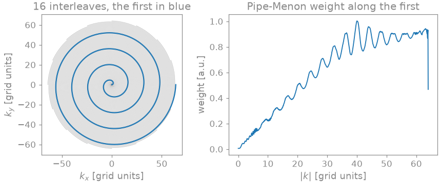
bartorch.tools.traj() does not generate spirals, so you write one yourself: sixteen Archimedean interleaves reaching \(\pm n/2\), each with \(n/32\) turns so that neighbouring turns of the whole set are one grid unit apart (the Nyquist spacing), and 1024 samples per interleaf.

INTERLEAVES, READOUT = 16, 1024

progress = torch.linspace(0.0, 1.0, READOUT)
radius = SIZE / 2 * progress
turns = SIZE / (2 * INTERLEAVES)
arms = []
for arm in range(INTERLEAVES):
    angle = 2 * torch.pi * (turns * progress + arm / INTERLEAVES)
    kx, ky = radius * torch.cos(angle), radius * torch.sin(angle)
    arms.append(torch.stack([kx, ky, torch.zeros(READOUT)], dim=-1))
spiral = torch.stack(arms)  # (interleaves, samples, 3)

spiral_samples = bartorch.nufft(image, spiral)
flat = spiral[..., :2].reshape(-1, 2)
spiral_density = bartorch.estimate_density(flat, shape)
spiral_density = spiral_density.reshape(INTERLEAVES, READOUT, 1)
spiral_density = spiral_density.to(torch.complex64)

spiral_plain = bartorch.nufft_adjoint(spiral_samples, spiral, image_shape=shape)
spiral_compensated = bartorch.nufft_adjoint(
    spiral_samples * spiral_density, spiral, image_shape=shape
)
spirals = {"no weights": spiral_plain, "Pipe-Menon": spiral_compensated}
for name, adjoint in spirals.items():
    nrmse = bt.nrmse(image.abs(), adjoint.abs(), scaled=True)
    print(f"spiral, {name:>10}  NRMSE {nrmse:.3f}")

• 
• 

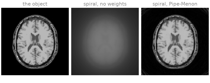
spiral, no weights  NRMSE 0.693
spiral, Pipe-Menon  NRMSE 0.089

The weight grows with \(\lvert k \rvert\): the interleaves stay a constant distance apart while each sample covers a longer stretch of arc, so the samples are densest at the centre. It ripples with the period of the turns, levels off in the outer part of k-space, and drops over the last samples, where the outermost turn has no neighbour outside it. Without the weights the spiral image is a low-contrast blur, as the radial one was; with them the tissue contrast and the edges are restored, and the NRMSE printed above drops accordingly.

The normal operator

An iterative reconstruction applies \(A^H A\) once per iteration, and for a NUFFT that costs a forward and an adjoint transform. Alternatively, \(A^H A\) is a convolution of the image with the PSF, which is computed once on a grid twice the size of the image [5] (the Toeplitz embedding). bartorch.linop.NUFFT is the transform as an operator, and A.gram() applies its normal operator as that convolution. The timing below compares both forms:

A = linop.NUFFT(golden, image_shape=shape)

repeats = 5
start = time.perf_counter()
for _ in range(repeats):
    toeplitz = A.gram()(image)
convolution = (time.perf_counter() - start) / repeats

start = time.perf_counter()
for _ in range(repeats):
    pair = A.H(A(image))
transforms = (time.perf_counter() - start) / repeats

difference = (toeplitz - pair).abs().max() / pair.abs().max()
print(f"A^H A as a convolution   {1e3 * convolution:6.1f} ms")
print(f"A^H A as two transforms  {1e3 * transforms:6.1f} ms")
print(f"relative difference      {float(difference):.1e}")

A^H A as a convolution      1.0 ms
A^H A as two transforms     0.9 ms
relative difference      2.7e-03

The two agree to a small multiple of the transform’s tolerance, and the convolution is the faster of the two.

The point spread function

bartorch.tools.psf() computes that PSF on its own: the adjoint reconstruction of a point object sampled along the trajectory. The reconstructed image is the object convolved with it. Compare the full scan with one of an eighth of the spokes:

full = bt.traj(readout=SIZE, spokes=SPOKES, radial=True, golden=True)
eighth = bt.traj(readout=SIZE, spokes=SPOKES // 8, radial=True, golden=True)
fully_sampled = bt.psf(full)
undersampled = bt.psf(eighth)

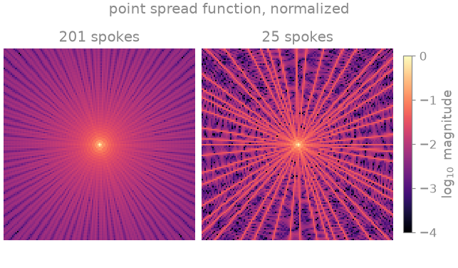
On a logarithmic scale, the PSF of the full scan is a sharp central peak on a low, even skirt. With an eighth of the spokes the skirt breaks up into bright lines radiating from the centre. Convolving the object with this PSF produces the streaks of an undersampled radial image.

Exercise: angular undersampling

Repeat the gridding reconstruction with the ramp weights for fewer and more spokes than 201, and compare the error and the images:

counts = (25, 50, 100, 201, 400)
scores, images = [], {}
for count in counts:
    trajectory = bt.traj(readout=SIZE, spokes=count, radial=True, golden=True)
    acquired = bartorch.nufft(image, trajectory)
    gridded = bartorch.nufft_adjoint(
        acquired * ramp(trajectory),
        trajectory,
        image_shape=shape,
    )
    scores.append(bt.nrmse(image.abs(), gridded.abs(), scaled=True))
    images[count] = gridded

• 
• 

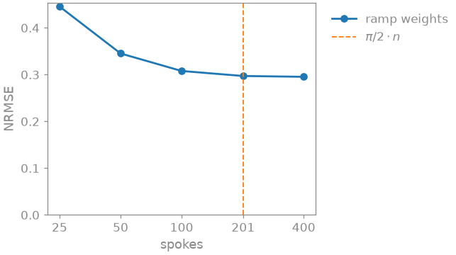
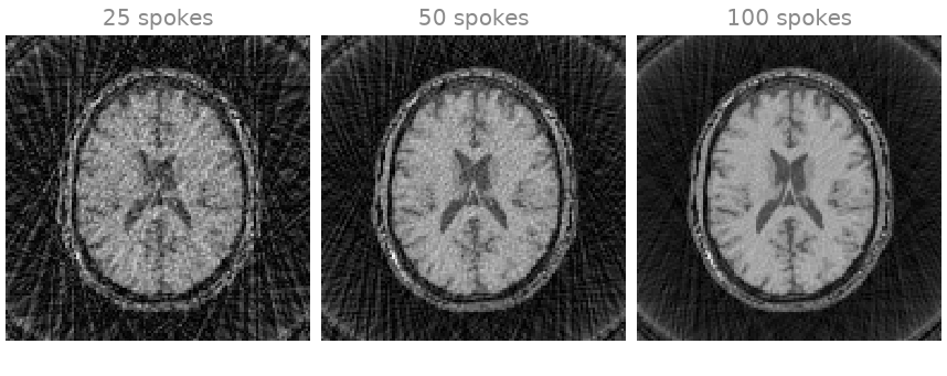
Below 201 spokes the error rises with every halving, and the images show why: streaks across the whole field of view, denser and brighter the fewer spokes you keep. Above 201 the error barely moves: undersampling no longer limits it, and what remains includes the corners of k-space the disc never covers. Try the same with uniform spokes (drop golden=True), or with fewer spiral interleaves.

As a spec

What this lesson built, stated the way you would ask an agent for it:

With bartorch, sample a 128x128 complex image along a 2D golden-angle
radial trajectory of 201 spokes of 128 samples (bt.traj, grid units),
with bartorch.nufft, and check one spoke against the explicit DFT in
float64. Reconstruct by gridding with bartorch.nufft_adjoint, without
weights, with the ramp |k| (clamped at 0.25) and with
bartorch.estimate_density, and report each NRMSE. Repeat for a
16-interleaf Archimedean spiral of 1024 samples. Time linop.NUFFT's
A.gram() against A.H(A(x)), and compare bt.psf for 201 and 25 spokes.

References

[1]

Collins DL, Zijdenbos AP, Kollokian V, Sled JG, Kabani NJ, Holmes CJ, Evans AC. Design and construction of a realistic digital brain phantom. IEEE Trans Med Imaging 17(3):463-468 (1998). https://doi.org/10.1109/42.712135

[2]

Barnett AH, Magland J, af Klinteberg L. A parallel nonuniform fast Fourier transform library based on an “exponential of semicircle” kernel. SIAM J Sci Comput 41(5):C479-C504 (2019). https://doi.org/10.1137/18M120885X

[3]

Winkelmann S, Schaeffter T, Koehler T, Eggers H, Doessel O. An optimal radial profile order based on the Golden Ratio for time-resolved MRI. IEEE Trans Med Imaging 26(1):68-76 (2007). https://doi.org/10.1109/TMI.2006.885337

[4] (1,2)

Pipe JG, Menon P. Sampling density compensation in MRI: rationale and an iterative numerical solution. Magn Reson Med 41(1):179-186 (1999). https://doi.org/10.1002/(SICI)1522-2594(199901)41:1%3C179::AID-MRM25%3E3.0.CO;2-V

[5]

Fessler JA, Lee S, Olafsson VT, Shi HR, Noll DC. Toeplitz-based iterative image reconstruction for MRI with correction for magnetic field inhomogeneity. IEEE Trans Signal Process 53(9):3393-3402 (2005). https://doi.org/10.1109/TSP.2005.853152