

Note
Go to the end to download the full example code.
11. Training an unrolled network#

In lesson 10 the proximal step of ADMM was a denoiser pretrained on photographs, never trained on MR images or on the residual aliasing of an undersampled scan. In this lesson you train the denoiser through the iteration: a fixed number of ADMM steps is unrolled into one network, which is fitted end to end against fully sampled images.
This is MoDL [2]. The encoding model, the SENSE operator \(A\) with its coil sensitivities, Fourier transform and sampling pattern, stays fixed, and the network is trained only for the part of the image that the data leave undetermined. As published, MoDL alternates a learned denoiser \(D_w\) and a data-consistency step (half-quadratic splitting):
The second line is a conjugate-gradient solve of \((A^H A + \lambda) x = A^H y + \lambda z^{k}\). ADMM [3] is the same splitting with a dual variable \(u\) carried along,
so MoDL is ADMM with \(u\) held at zero. The dual variable accumulates the mismatch between the data-consistent and the denoised image, so that a fixed point satisfies the data constraint rather than a penalized version of it.
bartorch.optim.ADMMBlock is one step of BART’s admm.c,
conjugate-gradient x-update included, and bartorch.learning.Unrolled
repeats it. The network enters the proximal step through
bartorch.priors.ImplicitPrior, as the pretrained one did in lesson
10, and \(\rho\) is trained with its weights.
Learning objectives
Put a network in the proximal step of
bartorch.optim.ADMMBlockthroughbartorch.priors.ImplicitPrior.Unroll the iteration with
bartorch.learning.Unrolledand train it end to end withlightning, on data held and augmented bytorchio.Cut the memory of a deeper unrolled network with checkpointing or per-iteration training.
Previous: 10. Plug-and-play reconstruction. Next: the Tours, where you continue with standalone topics; the learning workflows among them cover networks for complex volumes, staged and self-supervised training, annealed plug-and-play and uncertainty.
Training images#
You need fully sampled images to train against. Here they are 32 axial slices of one BrainWeb subject [1], rendered as \(T_1\)-weighted spin-echo images with a smooth phase, as in lesson 2; the code is hidden. You split them by position, not at random: the first 24 train and the last 8 validate, so that no validation slice has a near-duplicate neighbour in the training set.
One subject, 24 slices and one sampling pattern are a phantom, not a training set. The trained weights are not expected to generalise; the lesson is about the construction.
import lightning
import torch
import torchio

import bartorch
import bartorch.tools as bt

from bartorch import learning, linop, optim, priors
from monai.metrics import PSNRMetric, SSIMMetric
from torch.utils.data import DataLoader

_ = torch.manual_seed(0)

train_images = images[:24]
valid_images = images[24:]
print(f"{len(train_images)} slices to train, {len(valid_images)} to validate")
24 slices to train, 8 to validate
The acquisition#
Eight channels of BART’s analytical head coil and a variable-density random undersampling of the phase encodes, with the central 8 always acquired. The pattern is the same for every slice, so one operator serves the whole dataset. If each item had its own pattern, you would need one operator per item.
COILS = 8
ACCELERATION = 4
CENTRE = 8  # phase encodes always acquired

sensitivities = bt.coils(t=bt.grid(D=(SIZE, SIZE, 1)), n=COILS)[:, 0]
sensitivities /= bartorch.rss(sensitivities, axes=(0,), keepdim=True)

pattern = lines.to(torch.complex64)[:, None].expand(SIZE, SIZE).contiguous()

A = linop.CartesianSense(sensitivities, (SIZE, SIZE), pattern=pattern)
print(f"{int(lines.sum())} of {SIZE} phase encodes")
print(f"A: {A.ishape} -> {A.oshape}")
34 of 128 phase encodes
A: (128, 128) -> (8, 128, 128)
The k-space of a slice is \(A x\) plus complex Gaussian noise. A is
built for one image, so you apply it to a batch item by item. The blocks in
bartorch.optim do the same inside, which is why the network below
accepts a batch even though the operator does not. measure also returns
\(A^H y\), the image the unrolled network starts from.
NOISE = 0.005


def measure(images, generator=None):
    """Images, their noisy k-space and the adjoint reconstructions."""
    x = torch.stack(list(images))
    y = torch.stack([A(item) for item in x])
    noise = torch.randn(y.shape, dtype=torch.complex64, generator=generator)
    y = y + NOISE * noise
    return x, y, torch.stack([A.H(item) for item in y])
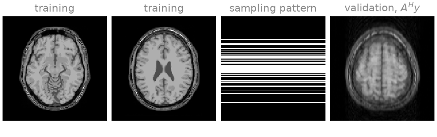
Two training slices, the sampling pattern (phase encoding vertical), and what the network starts from on a validation slice: \(A^H y\), with the aliasing of the random undersampling and the noise.
The dataset#
torchio holds the images and augments them. Its ScalarImage wants
a real tensor of shape (channels, width, height, depth);
bartorch.learning.as_real() and as_complex()
convert between that and a complex image, with the real and imaginary parts
as the two channels and the slice as a volume one voxel deep.
Why torchio and not a plain list? It draws one random transform per
subject and applies it to every image of that subject, so anything that has
to stay registered with the image (coil sensitivities, parameter maps) is
transformed with it. Here each subject holds one image, and the transform is
a flip and a rotation of at most eight degrees: the tissue the denoiser
learns stays the same, its orientation varies.
augmentation = torchio.Compose(
    [
        torchio.RandomFlip(axes=(0,), flip_probability=0.5),
        torchio.RandomAffine(
            scales=0,
            degrees=(0, 0, 0, 0, -8, 8),
            translation=0,
        ),
    ]
)


def subjects(images):
    return [
        torchio.Subject(image=torchio.ScalarImage(tensor=real))
        for real in (learning.as_real(image)[..., None] for image in images)
    ]


def collate(batch):
    """Simulate k-space for a batch of subjects."""
    planes = (subject["image"][torchio.DATA][..., 0] for subject in batch)
    return measure(learning.as_complex(plane) for plane in planes)


train_loader = DataLoader(
    torchio.SubjectsDataset(subjects(train_images), transform=augmentation),
    batch_size=2,
    shuffle=True,
    collate_fn=collate,
)
valid_loader = DataLoader(
    torchio.SubjectsDataset(subjects(valid_images)),
    batch_size=2,
    collate_fn=collate,
)
The network#
Three objects:
deepinv’sDnCNN[4], a residual convolutional denoiser of the family MoDL’s own five-layer network belongs to. It is a plainnn.Moduleon real images.ImplicitPriorpresents it as a regularization term.spatial=2, channels=2sets the layout: real and imaginary parts as two channels, the batch axes folded, and each image scaled to unit peak modulus around the call.Unrolledapplies the ADMM stepITERATIONStimes. One block is shared by every iteration, which is MoDL’s weight sharing, andrho, MoDL’s \(\lambda\), is made trainable.
alpha=1.0 turns off BART’s over-relaxation, so the step is the iteration
written at the top; cg_maxiter is the budget of the x-update, MoDL’s
ten conjugate-gradient steps.
from deepinv.models import DnCNN

ITERATIONS = 5  # unrolled steps, MoDL's K


def modl():
    """An unrolled network, and the block it shares."""
    network = DnCNN(in_channels=2, out_channels=2, depth=5, pretrained=None)
    prior = priors.ImplicitPrior(network, spatial=2, channels=2)
    block = optim.ADMMBlock(prior, rho=0.05, alpha=1.0, cg_maxiter=10)
    block.rho.requires_grad_()
    return learning.Unrolled(block, iterations=ITERATIONS), block


model, block = modl()
learned = sum(p.numel() for p in model.parameters() if p.requires_grad)
print(f"{learned} learned values, shared by all {ITERATIONS} iterations")
print(f"rho starts at {float(block.rho.detach()):.3f}")
113155 learned values, shared by all 5 iterations
rho starts at 0.050
Training#
lightning runs the loop, and the module is an ordinary supervised one:
a forward pass, a loss against the fully sampled image, and metrics from
monai. The loss is computed on a tensor and requires nothing of the
reconstruction that produced it. The gradient is propagated through the
denoiser, the conjugate-gradient solves and \(\rho\).
EPOCHS = 15

psnr = PSNRMetric(max_val=1.0)
ssim = SSIMMetric(spatial_dims=2, data_range=1.0)


class Reconstruction(lightning.LightningModule):
    """Supervised training of an unrolled network."""

    def __init__(self, model, lr=1e-3):
        super().__init__()
        self.model = model
        self.lr = lr

    def forward(self, y, start):
        return self.model(y, A, x0=start)

    def training_step(self, batch, index):
        x, y, start = batch
        loss = (self(y, start) - x).abs().square().mean()
        self.log("loss", loss, prog_bar=True)
        return loss

    def validation_step(self, batch, index):
        x, y, start = batch
        out = self(y, start).abs()[:, None]
        self.log("psnr", psnr(out, x.abs()[:, None]).mean(), prog_bar=True)
        self.log("ssim", ssim(out, x.abs()[:, None]).mean(), prog_bar=True)

    def configure_optimizers(self):
        return torch.optim.Adam(self.parameters(), lr=self.lr)


trainer = lightning.Trainer(
    max_epochs=EPOCHS,
    accelerator="cpu",
    logger=False,
    enable_checkpointing=False,
    enable_model_summary=False,
    gradient_clip_val=1.0,
)
trainer.fit(Reconstruction(model), train_loader, valid_loader)

print(f"rho ended at {float(block.rho.detach()):.3f}")
/opt/hostedtoolcache/Python/3.12.15/x64/lib/python3.12/site-packages/lightning/pytorch/utilities/_pytree.py:21: `isinstance(treespec, LeafSpec)` is deprecated, use `isinstance(treespec, TreeSpec) and treespec.is_leaf()` instead.
/opt/hostedtoolcache/Python/3.12.15/x64/lib/python3.12/site-packages/lightning/pytorch/trainer/connectors/data_connector.py:434: The 'val_dataloader' does not have many workers which may be a bottleneck. Consider increasing the value of the `num_workers` argument` to `num_workers=3` in the `DataLoader` to improve performance.
/opt/hostedtoolcache/Python/3.12.15/x64/lib/python3.12/site-packages/lightning/pytorch/trainer/connectors/data_connector.py:434: The 'train_dataloader' does not have many workers which may be a bottleneck. Consider increasing the value of the `num_workers` argument` to `num_workers=3` in the `DataLoader` to improve performance.
Epoch 14/14 ━━━━━━━━━━━━━━━━━ 12/12 0:00:16 • 0:00:00 0.74it/s loss: 0.000 psnr:
                                                               32.696 ssim:
                                                               0.885
rho ended at 0.027
Results#
You compare the trained network with three reconstructions of the same validation k-space: the adjoint it starts from; conjugate-gradient SENSE, which fits the data term alone; and the same ADMM iteration with a wavelet penalty in place of the network, run for fifty iterations rather than five.
torch.manual_seed(7)
truth, kspace, adjoint = measure(valid_images)

with torch.no_grad():
    unrolled = model(kspace, A, x0=adjoint)

cg = torch.stack([optim.cg(item, A, maxiter=30) for item in kspace])
wavelet = priors.Wavelet(axes=(-1, -2), weight=0.002)
admm = torch.stack(
    [optim.admm(item, A, wavelet, maxiter=50, rho=0.1) for item in kspace],
)


def quality(estimate):
    """Mean PSNR and SSIM of a batch of magnitudes against the truth."""
    a, b = estimate.abs()[:, None], truth.abs()[:, None]
    return float(psnr(a, b).mean()), float(ssim(a, b).mean())


rows = {
    "adjoint": adjoint,
    "CG SENSE": cg,
    "ADMM, wavelet": admm,
    f"MoDL, K={ITERATIONS}": unrolled,
}
for name, estimate in rows.items():
    made = quality(estimate)
    print(f"{name:>16}   PSNR {made[0]:5.2f} dB   SSIM {made[1]:.3f}")
      adjoint   PSNR 23.71 dB   SSIM 0.679
     CG SENSE   PSNR 29.69 dB   SSIM 0.681
ADMM, wavelet   PSNR 31.64 dB   SSIM 0.898
    MoDL, K=5   PSNR 32.70 dB   SSIM 0.884
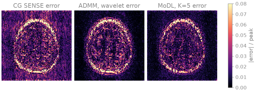
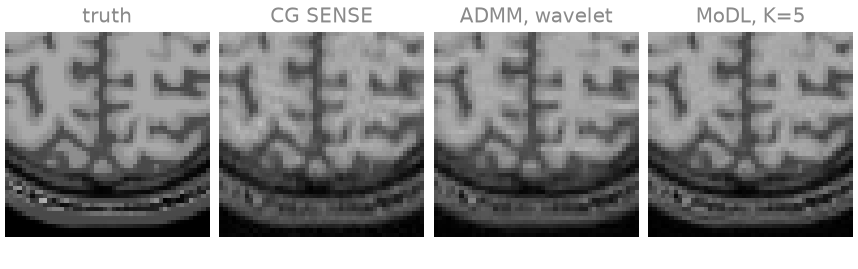
The error maps share one scale. CG SENSE removes most of the aliasing but amplifies the noise, which covers the whole field of view. The wavelet penalty and the unrolled network both suppress it, and both leave their largest errors at the bright, thin scalp. In the enlarged region the two differ little; the network has the higher PSNR, the wavelet penalty the slightly higher SSIM. Training also lowered \(\rho\) from 0.05 to about 0.026, which weights the network’s output less against the data in each x-update than at the start.
Do not read the table as a comparison of methods. Fifteen epochs over 24 slices of one subject, against a wavelet penalty with a hand-picked weight, says nothing about either on measured data. For that you would need many subjects, validation on subjects left out of training, and a fixed reconstruction time.
Deeper unrolled stack#
Five iterations of a 2D encoding record a computational graph of modest size. Ten iterations of a 3D non-Cartesian encoding do not, and the memory is dominated by the denoiser. The backward pass of an operator is one more application of that operator and stores nothing that grows with the iteration count; a convolutional network stores every activation, once per iteration.
Unrolled provides two alternatives, neither of
which changes the forward value (Learned reconstruction):
detach=Truestarts each iteration from a detached state, so the graph spans one iteration. With a loss on each image thatsteps()yields, that is greedy per-iteration training, and its memory does not depend on the iteration count.checkpoint=Truekeeps only the states between iterations and recomputes the interior of each step during the backward pass. The gradient is the end-to-end one, and each block is applied twice.
Pretraining the denoiser alone, then greedy per-iteration training, then end-to-end fine-tuning with checkpointing is the staged schedule reported for a fully 3D unrolled reconstruction [5]; the Tour Staged training of an unrolled network follows it. Greedy training does not suit the ADMM step: its image is the x-update, which depends on the denoiser only through the previous iteration’s auxiliary variable, and a detached start cuts that dependence. That Tour uses a proximal-gradient step instead, whose image is the denoiser’s output.
Compare the gradient of rho with and without checkpointing. rho
enters every iteration and every conjugate-gradient solve, so its gradient
is propagated through all of them:
x, y, start = measure(valid_images[:1])
made = []

for recompute in (False, True):
    stack = learning.Unrolled(
        block,
        iterations=ITERATIONS,
        checkpoint=recompute,
    )
    for parameter in stack.parameters():
        parameter.grad = None
    (stack(y, A, x0=start) - x).abs().square().mean().backward()
    made.append(float(block.rho.grad))

print(f"rho's gradient: {made[0]:.6g} recorded, {made[1]:.6g} recomputed")
rho's gradient: 0.000585573 recorded, 0.000585573 recomputed
The two gradients agree to every printed digit: checkpointing changes the memory, not the result.
A third alternative is not to unroll. bartorch.optim.FixedPoint
runs the block to its fixed point and differentiates there, by solving the
adjoint fixed-point equation, so its memory is that of one step whatever
the iteration count. That is a deep-equilibrium model [6], and the
stack you trained is its truncated form.
Exercise: iterations beyond training#
The block was trained for five iterations. Wrap the same trained block in
a new Unrolled with fewer or more iterations
and evaluate it on the validation slices; this needs forward passes only.
depths = (1, 2, 3, 5, 8, 12)
scores = []
with torch.no_grad():
    for depth in depths:
        stack = learning.Unrolled(block, iterations=depth)
        scores.append(quality(stack(kspace, A, x0=adjoint))[0])
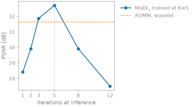
PSNR rises up to the five iterations the block was trained for and falls
beyond them: at 8 and 12 iterations it is below the wavelet penalty again.
Training fitted the block to the iterates of a five-step stack and
constrained nothing after the fifth, so the unrolled network is not a
convergent iteration. If the iteration count has to be free at inference,
FixedPoint is the formulation that trains for it.
As a spec#
What this lesson built, stated the way you would ask an agent for it:
Train a MoDL-style unrolled reconstruction for 2D Cartesian SENSE
(128x128, 8 coils, variable-density pattern of 34 of 128 lines including
the central 8, known sensitivities, k-space noise 0.005) with bartorch.
Wrap deepinv's
DnCNN (2 in/out channels, depth 5, untrained) as
priors.ImplicitPrior(spatial=2, channels=2), put it in
optim.ADMMBlock(rho=0.05, alpha=1.0, cg_maxiter=10) with rho trainable,
and unroll 5 iterations with learning.Unrolled. Hold the images in
torchio (random flip, rotation up to 8 degrees), simulate k-space in the
collate function, and train with lightning (Adam, lr 1e-3, 15 epochs,
batch 2, squared error against the fully sampled image, monai PSNR and
SSIM on validation). Compare against CG SENSE and wavelet ADMM, and check
that checkpoint=True reproduces the gradient of rho.
References#
Total running time of the script: (5 minutes 1.130 seconds)