Readout oversampling and apodization

In this tour you apply two corrections to Cartesian k-space before reconstruction. The readout is usually sampled at twice the density the matrix requires; removing that oversampling gives the image the prescribed matrix. And the truncation of k-space at the edge of the acquired matrix causes Gibbs ringing next to every sharp edge, which an apodization window reduces at the cost of resolution.

You work on a Shepp-Logan phantom whose k-space is evaluated analytically at the sample positions, so the oversampling and the truncation are those of a continuous object and not of a pixel grid.

Prerequisites: lesson 1, 1. Your data as tensors.

Learning objectives

• Remove readout oversampling with bartorch.remove_readout_oversampling(), and see why that is not the same as dropping the outer readout samples.

• Relate the Gibbs ringing of a truncated acquisition to the side lobes of its point spread function.

• Apodize k-space with bartorch.apodize() and measure what you pay in resolution for the ringing you remove.

• Choose between a radial and a separable window.

import math

import torch

import bartorch
import bartorch.tools as bt

Readout oversampling

The receiver digitises the echo at twice the rate your matrix requires, so that its anti-aliasing filter can roll off outside the field of view. Twofold oversampling halves the sample spacing \(\Delta k_x\), and so doubles the field of view along the readout. The extent of k-space, and with it the resolution, stays the same.

Your acquisition has 128 phase-encoding lines and 256 readout samples at half the phase-encoding spacing, in the grid units of a 128 matrix. The first trajectory component is \(k_x\), along the last image axis.

MATRIX = 128
phase_encodes = (torch.arange(MATRIX) - MATRIX // 2).float()
readout = (torch.arange(2 * MATRIX) - MATRIX).float() / 2
ky, kx = torch.meshgrid(phase_encodes, readout, indexing="ij")
trajectory = torch.stack([kx, ky, torch.zeros_like(kx)], dim=-1)

oversampled = bt.phantom(traj=trajectory).reshape(MATRIX, 2 * MATRIX)


def image_of(kspace):
    return bartorch.fft(kspace, axes=(-2, -1), inverse=True).abs()

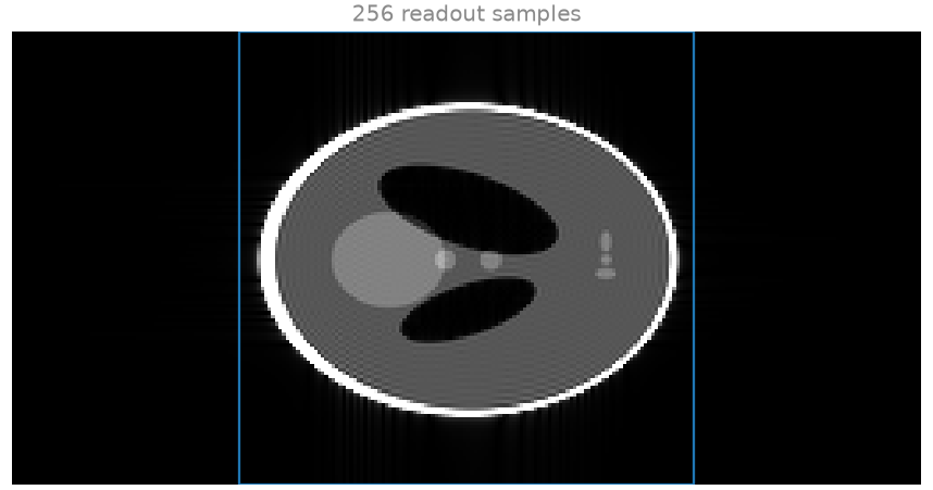
The image is twice as wide as you asked for, and the object sits in the middle half of it, inside the box. That box is what you want to keep.

bartorch.remove_readout_oversampling() transforms the readout to the image domain, crops the field of view to your matrix and transforms back. The tempting shortcut, keeping only the central 128 readout samples, does something else: it keeps the doubled field of view and halves the resolution along the readout. You compare both with an acquisition made without oversampling. The crop uses the unitary transform, whose scale depends on the number of samples, so you divide by \(\sqrt{2}\), the square root of the ratio of the two transform lengths.

cropped = bartorch.remove_readout_oversampling(oversampled, MATRIX, axis=-1)
cropped = cropped / math.sqrt(2)
truncated = bartorch.resize(oversampled, (MATRIX, MATRIX)) / math.sqrt(2)
reference = bt.phantom(MATRIX, kspace=True)

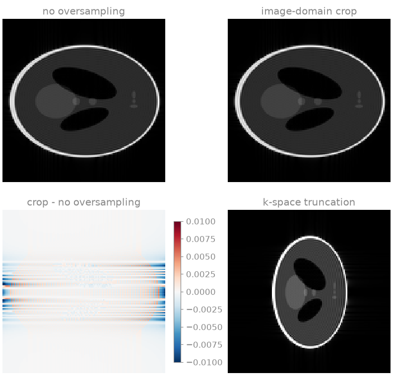
crop against no oversampling: NRMSE 4.8e-03

The crop reproduces the acquisition without oversampling to within a few parts in a thousand. What is left, in the difference panel, is the part of the truncation ringing that spread past your field of view along the readout and was cropped away with it. Dropping k-space samples instead widens the pixel to twice its size along \(x\): the object shrinks to half of the matrix.

Apodization

An acquisition that stops at the edge of k-space is the object’s spectrum multiplied by a rectangle, so its image is the object convolved with a sinc. The first side lobe of the sinc is 22 % of its peak; at a step edge you see it as an overshoot of about 9 % and as ringing that dies out over a few pixels. An apodization window rolls the data off towards the edge of k-space: the side lobes drop and the main lobe of the point spread function widens [1].

You acquire the phantom on a 64 matrix and reconstruct it on a 128 grid by zero-filling, which interpolates the image and lets you see the ringing between the pixels of the acquired grid.

GRID, ACQUIRED = 128, 64
image = bt.phantom(GRID).abs()
measured = bt.phantom(ACQUIRED, kspace=True)


def reconstruct(kspace):
    padded = bartorch.resize(kspace, (GRID, GRID))
    return bartorch.fft(padded, axes=(-2, -1), inverse=True).abs()

You try two windows. bartorch.fermi_window() lets you set the radius of its half height and the width of its transition separately, and keeps a wide flat passband. bartorch.hann_window() tapers all the way from the centre of k-space to zero at the edge.

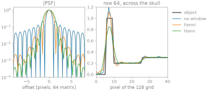
To see the side lobes you evaluate each point spread function on a grid eight times finer than the acquired one: without a window the sinc has its zeros exactly at the pixels of the acquired grid, so read off that grid it shows no side lobes at all.

fermi = bartorch.fermi_window((ACQUIRED, ACQUIRED), radius=0.8, width=0.08)
hann = bartorch.hann_window((ACQUIRED, ACQUIRED))
windows = {
    "no window": torch.ones(ACQUIRED, ACQUIRED),
    "Fermi": fermi,
    "Hann": hann,
}

UPSAMPLE = 8
FINE = UPSAMPLE * ACQUIRED
offset = (torch.arange(FINE) - FINE // 2) / UPSAMPLE  # in acquired pixels


def psf(window):
    fine = bartorch.resize(window.to(torch.complex64), (FINE, FINE))
    plane = bartorch.fft(fine, axes=(-2, -1), inverse=True).abs()
    profile = plane[FINE // 2]
    return profile / profile.max()

bartorch.apodize() multiplies k-space by either window over the axes you name:

fermi_k = bartorch.apodize(measured, kind="fermi", radius=0.8, width=0.08)
hann_k = bartorch.apodize(measured, kind="hann")
reconstructions = {
    "no window": reconstruct(measured),
    "Fermi": reconstruct(fermi_k),
    "Hann": reconstruct(hann_k),
}

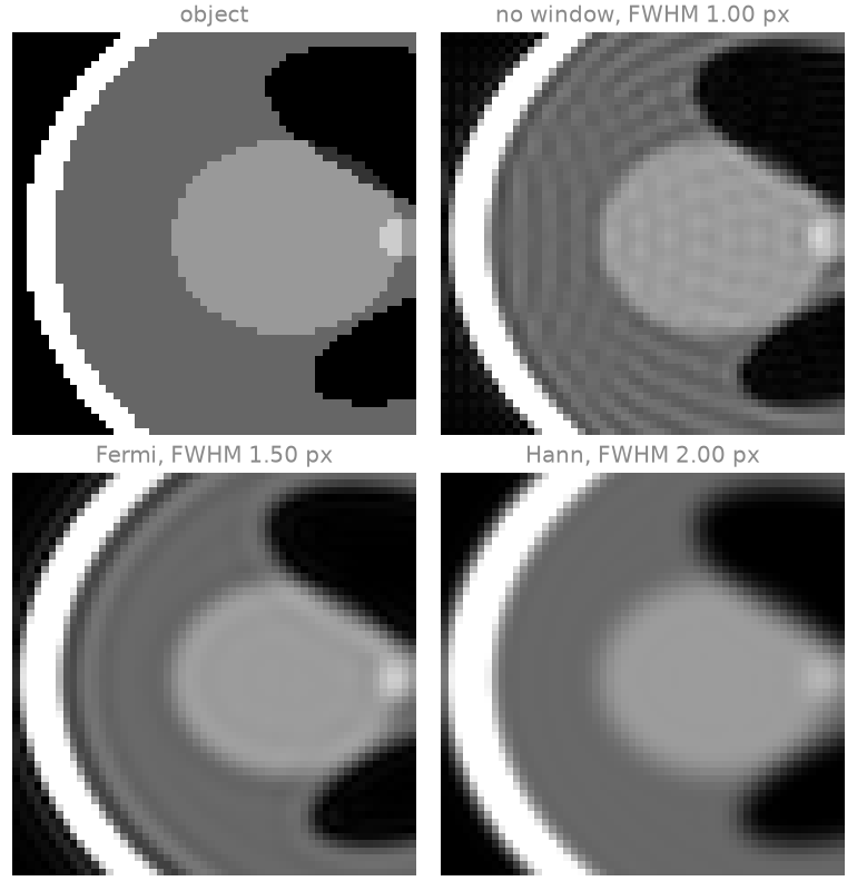
You measure the ringing as the standard deviation of the image over the uniform tissue within six pixels of the skull, and the resolution as the full width at half maximum (FWHM) of the point spread function, in pixels of the acquired grid. The side lobe column is the largest value of the point spread function beyond three pixels from its centre.

• 
• 

   window  ringing  side lobe     FWHM
no window   0.0404    9.1e-02   1.00 px
    Fermi   0.0325    2.6e-02   1.50 px
     Hann   0.0100    5.6e-03   2.00 px

The zoomed panels show the left edge of the skull, displayed from zero to half the skull intensity. Without a window you see the ringing as bands parallel to the skull running into the tissue next to it. The Fermi window lowers the far side lobes by a factor of three and the ringing next to the skull by about a fifth, and widens the point spread function by half a pixel. The Hann window removes the ringing almost entirely but doubles the FWHM, and the skull blurs into the tissue beside it. That is why the Fermi window, with its wide passband, is the usual compromise for anatomical imaging.

Radial and separable windows

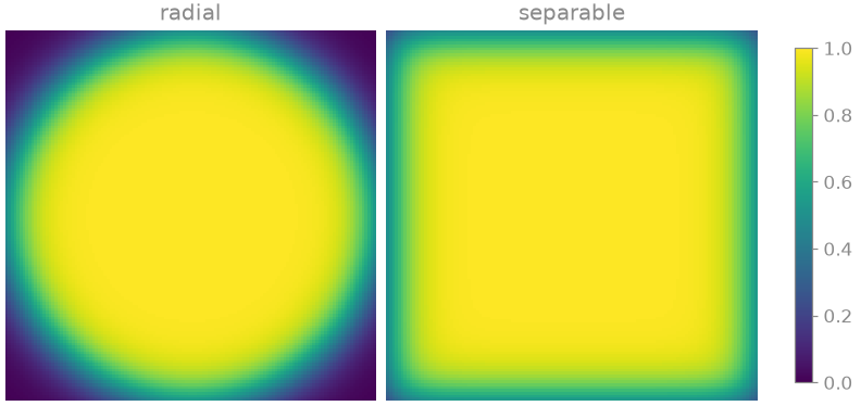
A window is a one-dimensional kernel, and there are two ways to spread it over 2D or 3D k-space. geometry="radial" evaluates it on the Euclidean norm of the normalized coordinates, which gives an ellipse. geometry="separable" multiplies the kernel along each axis, which keeps more of the corners of k-space.

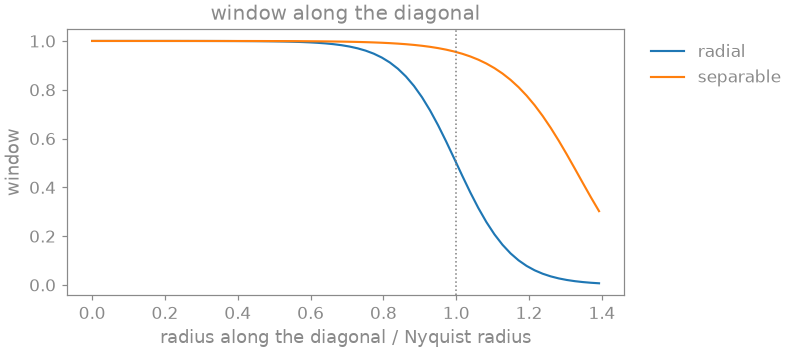
Bernstein et al. [1] give the ratio of the two at the diagonal Nyquist point as 52.4 % in two dimensions and 50.7 % in three, for a Fermi window of transition width 10/128. You can check that number: the radial window is 0.5 there, and the separable one is the product of the 1D kernel at \(1/\sqrt{d}\) along each of \(d\) axes. The 1D kernel at \(u\) is the window at the centre of a small grid with its radius moved to \(1 - u\).

TRANSITION = 10.0 / 128


def kernel(u):
    window = bartorch.fermi_window((4, 4), radius=1.0 - u, width=TRANSITION)
    return float(window[2, 2])


for dimensions in (2, 3):
    separable = kernel(1 / math.sqrt(dimensions)) ** dimensions
    ratio = 100 * 0.5 / separable
    print(f"{dimensions}D: radial / separable at the diagonal {ratio:.1f} %")

• 
• 

2D: radial / separable at the diagonal 52.4 %
3D: radial / separable at the diagonal 50.7 %

Both reproduce the published ratios. Along the diagonal the separable window stays near one for longer and reaches the Nyquist radius at about twice the radial window’s value. The radial window gives you the more isotropic point spread function and the higher signal-to-noise ratio; the separable one the better resolution along the diagonals. Both normalize each axis to its own Nyquist edge, so a rectangular matrix gets an ellipse matched to its grid.

Exercise: Fermi transition width

The Fermi window has two knobs. Keep its radius at 0.8 and sharpen or soften its transition, and watch the ringing next to the skull trade against the FWHM:

shape = (ACQUIRED, ACQUIRED)
for width in (0.02, 0.05, 0.08, 0.15):
    apodized = bartorch.apodize(measured, kind="fermi", radius=0.8, width=width)
    window = bartorch.fermi_window(shape, radius=0.8, width=width)
    ringing = float(reconstruct(apodized)[ringing_region].std())
    spread = fwhm(psf(window))
    print(f"width {width:.2f}: ringing {ringing:.4f}, FWHM {spread:.2f} px")

width 0.02: ringing 0.0532, FWHM 1.75 px
width 0.05: ringing 0.0432, FWHM 1.50 px
width 0.08: ringing 0.0325, FWHM 1.50 px
width 0.15: ringing 0.0165, FWHM 1.50 px

The FWHM is read on a grid of eighth pixels, so it moves in steps of 0.125. A soft transition lowers the ringing without moving the FWHM off 1.5 px. A sharp one does not bring you back to no window: with the radius at 0.8 it is a rectangle that cuts k-space at 80 % of its extent, so you get the ringing of a truncation and a wider point spread function on top of it.

As a spec

What this tour built, stated the way you would ask an agent for it:

For a 2D Cartesian k-space with twofold readout oversampling along the
last axis, remove the oversampling with
bartorch.remove_readout_oversampling(kspace, matrix, axis=-1) and check
it against an acquisition without oversampling. Then apodize a 64x64
k-space with bartorch.apodize (kind "fermi", radius 0.8, width 0.08, and
kind "hann"), zero-fill to 128, and report for each window the ringing
(standard deviation over uniform tissue next to the skull), the largest
point-spread-function side lobe beyond 3 pixels and the FWHM in acquired
pixels.

References

[1] (1,2)

Bernstein MA, Fain SB, Riederer SJ. Effect of windowing and zero-filled reconstruction of MRI data on spatial resolution and acquisition strategy. J Magn Reson Imaging 14(3):270-280 (2001). https://doi.org/10.1002/jmri.1183