Staged training of an unrolled network

In lesson 11 you trained an unrolled network end to end, which keeps the activations of every iteration in memory for the backward pass. For a 2D slice that memory is affordable; for a 3D volume, or a series of them, it exceeds a single GPU. In this tour you train an unrolled network for fourfold undersampled, eight-channel Cartesian brain data in three stages whose memory is bounded by one iteration, and you check that it removes the residual aliasing and the g-factor noise that CG-SENSE leaves at this acceleration.

The iteration is BART’s iterative soft thresholding with the thresholding replaced by a convolutional network \(D_\theta\),

\[x^{k+1} = D_\theta\!\left(x^{k} - \tau\, A^H (A x^{k} - y),\; k\right),\]

where \(A\) is the SENSE encoding (coil sensitivities, Fourier transform, sampling pattern) and \(\tau\) a learned step size. One set of weights serves every iteration. The iteration index \(k\) enters the network by feature-wise modulation (FiLM), so the same weights can remove the strong incoherent aliasing of the first iterates and the fine residual noise of the last.

Urman et al. [1] reach the end-to-end result in three stages:

1. Denoiser pretraining. The network alone learns to map degraded images to the fully sampled reference, each image tagged with the iteration index at which the unrolled iteration will meet that level of degradation.

2. Greedy training. Each iteration’s loss is back-propagated before the next iteration runs [2].

3. End-to-end fine-tuning. One loss on the final image, through the whole stack, with each iteration recomputed during the backward pass (gradient checkpointing) instead of stored.

bartorch.learning.Reconstruction runs each stage in lightning, and torchio holds and augments the training images.

Prerequisites: lesson 11, 11. Training an unrolled network.

Learning objectives

• Condition a bartorch.learning.UNet on the iteration index and pass the index to it through bartorch.priors.ImplicitPrior.

• Train an unrolled bartorch.optim.ISTBlock in the three stages of bartorch.learning.Reconstruction.

• Split a dataset by subject and augment it with transforms that preserve the complex MR signal.

Training without a reference trains the same network without fully sampled references.

Images and acquisition

Your images are axial slices of two BrainWeb subjects [3], simulated as \(T_1\)-weighted spin-echo images (TR 600 ms, TE 12 ms) with a smooth background phase, as in lesson 11. You split training and validation by subject: no slice of subject 4 is trained on, so the validation scores measure how a network trained on one head generalizes to another. A random split of slices would put neighbouring, nearly identical slices of the same head on both sides and overstate the result.

import lightning
import torch
import torchio

import bartorch
import bartorch.tools as bt

from bartorch import learning, linop, optim, priors
from monai.metrics import PSNRMetric, SSIMMetric
from torch.utils.data import DataLoader

COILS = 8
ITERATIONS = 4
ACCELERATION = 4
NOISE = 0.02

_ = torch.manual_seed(0)

train_images = brain_slices(subject=0, count=24)
valid_images = brain_slices(subject=4, count=8)

The acquisition is an eight-channel receive array with variable-density Cartesian undersampling of the phase encodes at \(R = 4\), around a fully sampled centre of eight lines. Complex Gaussian noise of standard deviation 0.02 (relative to an image peak of one) goes into k-space, an SNR at which the unfolding of CG-SENSE amplifies the noise visibly.

coils = bt.coils(t=bt.grid(D=(SIZE, SIZE, 1)), n=COILS)[:, 0]
sensitivities = coils / bartorch.rss(coils, axes=(0,), keepdim=True)

ky = torch.arange(SIZE) - SIZE / 2
density = torch.exp(-0.5 * (ky / (SIZE / 6)) ** 2)
chance = density / density.sum() * (SIZE / ACCELERATION)
draw = torch.rand(SIZE, generator=torch.Generator().manual_seed(1))
lines = draw < chance
lines[SIZE // 2 - 4 : SIZE // 2 + 4] = True
pattern = lines.to(torch.complex64)[:, None].expand(SIZE, SIZE).contiguous()
A = linop.CartesianSense(sensitivities, (SIZE, SIZE), pattern=pattern)

print(f"{len(train_images)} slices of subject 0, {len(valid_images)} of 4")
print(f"{int(lines.sum())} of {SIZE} phase encodes")

24 slices of subject 0, 8 of 4
24 of 96 phase encodes

Dataset

Each torchio subject holds one reference image as two real channels. Pick augmentations that turn one MR image into another the scanner could have produced: RandomGain applies a random receiver gain and global phase (a complex scale within 20 per cent in magnitude), and a flip and a small in-plane rotation vary the head’s orientation. You simulate k-space from the augmented reference in the collate function, so the measured data stay consistent with it. torchio’s intensity transforms, such as a gamma correction, act on the real and imaginary channels independently and would break that consistency.

A batch is a list of dictionaries, the form Reconstruction takes: the data, the operator, the reference, and the adjoint reconstruction the iteration starts from.

augmentation = torchio.Compose(
    [
        learning.RandomGain(log_scale=0.2),
        torchio.RandomFlip(axes=(0,), flip_probability=0.5),
        torchio.RandomAffine(
            scales=0,
            degrees=(0, 0, 0, 0, -8, 8),
            translation=0,
        ),
    ]
)


def subjects(images):
    made = []
    for x in images:
        image = torchio.ScalarImage(tensor=learning.as_real(x)[..., None])
        made.append(torchio.Subject(image=image))
    return made


def measured(x, generator=None):
    """One item: k-space of ``x``, the operator, the reference, ``A^H y``."""
    noise = torch.randn(A.oshape, dtype=torch.complex64, generator=generator)
    y = A(x) + NOISE * noise
    return {"y": y, "A": A, "target": x, "x0": A.H(y)}


def collate(batch):
    images = [s["image"][torchio.DATA][..., 0] for s in batch]
    return [measured(learning.as_complex(x)) for x in images]


train_loader = DataLoader(
    torchio.SubjectsDataset(subjects(train_images), transform=augmentation),
    batch_size=4,
    shuffle=True,
    collate_fn=collate,
)
generator = torch.Generator().manual_seed(2)
valid_items = [measured(x, generator) for x in valid_images]
valid_loader = DataLoader(valid_items, batch_size=4, collate_fn=list)

Network

The network is a 2D UNet on the real and imaginary planes, conditioned on the iteration index (steps=True). ComplexNet lays the complex image out as those planes and scales it to unit peak around the call. The U-Net is residual and starts as the identity, so the untrained stack is plain gradient descent. ImplicitPrior with step=True passes each iteration’s index to it.

network = learning.UNet(2, spatial=2, widths=(16, 32, 64), steps=True)
prior = priors.ImplicitPrior(learning.ComplexNet(network, spatial=2), step=True)
block = optim.ISTBlock(prior, step=1.0)
block.step.requires_grad_()

weights = sum(p.numel() for p in network.parameters())
print(f"{weights} weights, {2 * weights / 1e6:.2f} MB in half precision")

235730 weights, 0.47 MB in half precision

The three stages differ only in the model and the data you hand lightning; the trainer is the same each time:

def trainer(epochs):
    return lightning.Trainer(
        max_epochs=epochs,
        accelerator="cpu",
        logger=False,
        enable_checkpointing=False,
        enable_model_summary=False,
        enable_progress_bar=False,
    )

Stage 1: denoiser pretraining

The inputs are reconstructions of increasing quality – the zero-filled coil combination \(A^H y\), and CG-SENSE after 2, 5 and 20 iterations – each paired with the fully sampled reference and with the iteration index at which the unrolled network is expected to meet an image of that quality. You compute the pairs once; neither the unrolling nor the encoding enters this stage, which makes it the cheapest of the three.

STAGES = {0: 0, 2: 1, 5: 2, 20: 3}  # CG iterations -> iteration index

pairs = []
for x in train_images:
    item = measured(x)
    for iterations, index in STAGES.items():
        if iterations == 0:
            degraded = item["x0"]
        else:
            degraded = optim.cg(item["y"], A, maxiter=iterations)
        pairs.append({"input": degraded, "target": x, "step": index})

denoiser = learning.ComplexNet(network, spatial=2)
stage = learning.Reconstruction(denoiser, "denoiser", lr=2e-3)
trainer(15).fit(
    stage,
    DataLoader(pairs, batch_size=8, shuffle=True, collate_fn=list),
    DataLoader(pairs[:16], batch_size=8, collate_fn=list),
)

/opt/hostedtoolcache/Python/3.12.15/x64/lib/python3.12/site-packages/lightning/pytorch/utilities/_pytree.py:21: `isinstance(treespec, LeafSpec)` is deprecated, use `isinstance(treespec, TreeSpec) and treespec.is_leaf()` instead.
/opt/hostedtoolcache/Python/3.12.15/x64/lib/python3.12/site-packages/lightning/pytorch/trainer/connectors/data_connector.py:434: The 'val_dataloader' does not have many workers which may be a bottleneck. Consider increasing the value of the `num_workers` argument` to `num_workers=3` in the `DataLoader` to improve performance.
/opt/hostedtoolcache/Python/3.12.15/x64/lib/python3.12/site-packages/lightning/pytorch/trainer/connectors/data_connector.py:434: The 'train_dataloader' does not have many workers which may be a bottleneck. Consider increasing the value of the `num_workers` argument` to `num_workers=3` in the `DataLoader` to improve performance.

Stage 2: greedy training

detach=True starts every iteration from a detached state, and the greedy stage back-propagates each iteration’s loss before the next iteration runs, so memory holds one iteration. The losses are weighted geometrically along the stack, the last ten times the first, since the last image is the one you deliver. The network now sees its own iterates, which the CG-SENSE images of stage 1 only approximated.

To follow the stages you score the magnitude of each reconstruction of the validation slices by its mean PSNR and SSIM:

psnr = PSNRMetric(max_val=1.0)
ssim = SSIMMetric(spatial_dims=2, data_range=1.0)
truth = torch.stack(valid_images)


def quality(images):
    made, reference = images.abs()[:, None], truth.abs()[:, None]
    return (
        float(psnr(made, reference).mean()),
        float(ssim(made, reference).mean()),
    )


def reconstruct(model):
    with torch.no_grad():
        return torch.stack([model(i["y"], A, i["x0"]) for i in valid_items])


greedy = learning.Unrolled(block, iterations=ITERATIONS, detach=True)
scores = {"untrained": None}
scores["denoiser pretrained"] = quality(reconstruct(greedy))

trainer(8).fit(
    learning.Reconstruction(greedy, "greedy", lr=1e-3),
    train_loader,
    valid_loader,
)
scores["greedy"] = quality(reconstruct(greedy))

Stage 3: end-to-end training

The loss is now on the final image alone, so the earlier iterations are free to produce whatever intermediate image serves the last one best. checkpoint=True stores only the image between iterations and recomputes each iteration’s activations during the backward pass: the gradient is the exact end-to-end one, at the memory of those images plus one iteration.

stack = learning.Unrolled(block, iterations=ITERATIONS, checkpoint=True)
trainer(4).fit(
    learning.Reconstruction(stack, "end-to-end", lr=3e-4),
    train_loader,
    valid_loader,
)
scores["end to end"] = quality(reconstruct(stack))

Results

Two baselines frame the scores. The untrained stack is four gradient steps from \(A^H y\), since the residual network starts as the identity. CG-SENSE with twenty iterations is the reconstruction without a learned prior.

identity = priors.ImplicitPrior(lambda v: v)
gradient_steps = optim.ISTBlock(identity, step=1.0)
untrained = learning.Unrolled(gradient_steps, iterations=ITERATIONS)
scores["untrained"] = quality(reconstruct(untrained))
cg = torch.stack([optim.cg(i["y"], A, maxiter=20) for i in valid_items])
scores["CG SENSE, 20 iterations"] = quality(cg)

               untrained   PSNR 26.45 dB   SSIM 0.654
     denoiser pretrained   PSNR 26.32 dB   SSIM 0.913
                  greedy   PSNR 28.16 dB   SSIM 0.795
              end to end   PSNR 29.06 dB   SSIM 0.839
 CG SENSE, 20 iterations   PSNR 24.30 dB   SSIM 0.558
learned step: 1.139

Each stage starts from the weights the previous one left, and each raises the PSNR over the one before, from about 26.5 dB for the untrained stack to about 29.8 dB end to end, against about 24.3 dB for CG-SENSE. The pretrained denoiser has the highest SSIM and a low PSNR: inside the iteration it meets its own iterates rather than the CG-SENSE images it was trained on, and the greedy stage adapts it to them. With one training subject and a few epochs per stage, the numbers show the ordering of the stages, not what each reaches on a real dataset.

• 
• 

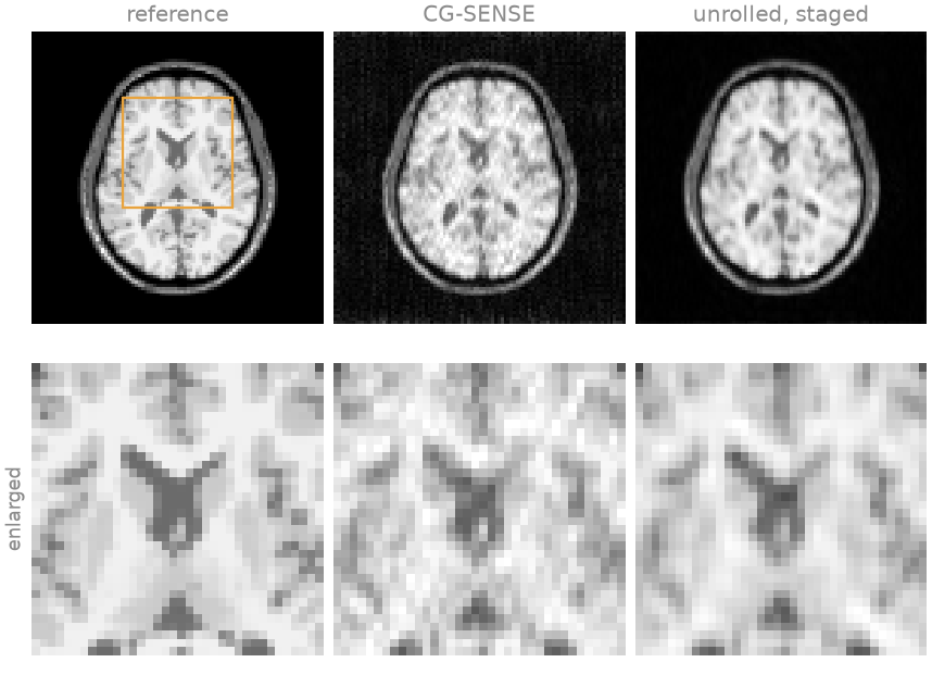
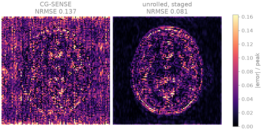
CG-SENSE at \(R = 4\) keeps a grainy, spatially varying noise – the g-factor amplification of the coil unfolding – and faint aliasing along the phase-encode direction (vertical). The unrolled network removes both; its error is concentrated at tissue boundaries, where it slightly smooths the cortex.

Checkpoints

Store the weights in half precision: that halves the file and loses nothing a float16 or bfloat16 inference would keep. load_state_dict casts them back to the network’s precision.

compact = {name: value.half() for name, value in stack.state_dict().items()}

fresh = learning.UNet(2, spatial=2, widths=(16, 32, 64), steps=True)
fresh_denoiser = learning.ComplexNet(fresh, spatial=2)
fresh_prior = priors.ImplicitPrior(fresh_denoiser, step=True)
restored = learning.Unrolled(optim.ISTBlock(fresh_prior), iterations=ITERATIONS)
restored.load_state_dict(compact)
print(f"restored: PSNR {quality(reconstruct(restored))[0]:5.2f} dB")

restored: PSNR 29.06 dB

Exercise: per-iteration gain

steps() yields the image after every iteration, so you can watch the trained stack and the untrained one converge. No training is involved:

curves = {}
for name, model in (("staged", stack), ("untrained", untrained)):
    with torch.no_grad():
        runs = [list(model.steps(i["y"], A, i["x0"])) for i in valid_items]
    iterates = [torch.stack(images) for images in zip(*runs)]
    curves[name] = [quality(images)[0] for images in iterates]

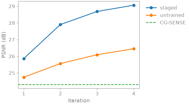
The staged stack improves the PSNR at every iteration, and its first iterate already scores above the fourth iterate of the untrained stack. The untrained stack is gradient descent on the data term, and its four steps also score above twenty iterations of CG-SENSE.

As a spec

What this tour built, stated the way you would ask an agent for it:

Train an unrolled ISTA network for 2D Cartesian SENSE (8 coils, R = 4,
8 central lines, k-space noise 0.02) with bartorch: optim.ISTBlock with a
learned step over priors.ImplicitPrior(ComplexNet(UNet(2, spatial=2,
widths=(16, 32, 64), steps=True)), step=True), 4 iterations. Train in
three lightning stages with learning.Reconstruction: "denoiser" on A^H y
and CG-SENSE images after 2, 5, 20 iterations tagged with steps 0-3
(15 epochs); "greedy" with Unrolled(detach=True) (8 epochs); "end-to-end"
with Unrolled(checkpoint=True) (4 epochs). Train on subject 0 with
torchio RandomGain, flip and rotation, validate on subject 4, and report
PSNR and SSIM after each stage against CG-SENSE.

References

[1]

Urman Y, Nishimura M, Abraham DR, Cao X, Setsompop K. Fully 3D unrolled magnetic resonance fingerprinting reconstruction via staged pretraining and implicit gridding. Magn Reson Med 96(5):2516-2529 (2026). https://doi.org/10.1002/mrm.70500

[2]

Wang K, Kellman M, Sandino CM, Zhang K, Vasanawala SS, Tamir JI, Yu SX, Lustig M. Memory-efficient learning for high-dimensional MRI reconstruction. MICCAI 2021, LNCS 12906:461-470. https://doi.org/10.1007/978-3-030-87231-1_45

[3]

Collins DL, Zijdenbos AP, Kollokian V, Sled JG, Kabani NJ, Holmes CJ, Evans AC. Design and construction of a realistic digital brain phantom. IEEE Trans Med Imaging 17(3):463-468 (1998). https://doi.org/10.1109/42.712135