3. Coil sensitivities

In lesson 2 you estimated the coil sensitivities with ESPIRiT from a block of 24 central lines and passed them to pics without examining them. SENSE [1] solves

\[y_c = P F (S_c \, x)\]

for the image \(x\) with the sensitivities \(S_c\) taken as known. Whatever is wrong in \(S_c\) ends up in the image, as residual aliasing or as shading, however good the solver.

On a scanner the sensitivities come either from a separate low-resolution prescan or, as here, from the scan itself: a fully sampled block of lines at the centre of k-space, the autocalibration (ACS) region. In this lesson you estimate them in three ways, reconstruct with each, and then shrink the ACS region to see which of the three still works.

Learning objectives

• Estimate coil sensitivities with bartorch.tools.caldir(), bartorch.tools.ecalib() (ESPIRiT) and bartorch.tools.nlinv(), and use each in bartorch.apps.pics().

• Recognise what a poor set of maps does to a SENSE reconstruction.

• Explain why ESPIRiT needs an ACS region larger than its kernel, and why nonlinear inversion does not.

Previous: 2. From k-space to an image. Next: 4. Joint reconstruction of image and sensitivity maps, where you reconstruct the image and the sensitivities together and write that reconstruction out as an operator and a solver.

Simulated acquisition

The object is BART’s Shepp-Logan phantom, seen through BART’s analytical eight-channel head coil. As in lesson 1, you ask for its k-space directly (kspace=True) rather than transforming a sampled image, so the data do not share the discretization of the reconstructions below. Then you add complex Gaussian noise of variance 2 to every sample.

import torch

import bartorch
import bartorch.tools as bt

from bartorch import apps

SIZE = 128
COILS = 8
ACCELERATION = 3

clean = bt.phantom(SIZE, coils=COILS, kspace=True)
kspace = bt.noise(clean, n=2.0, s=3)

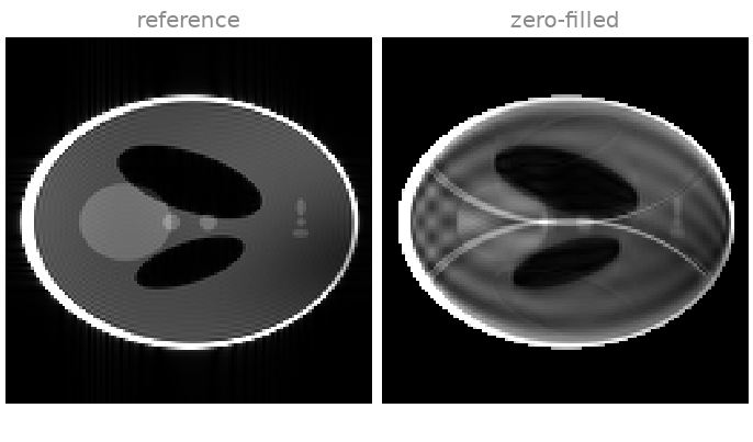
You acquire every third phase encode, plus a central block of calibration lines in full. Regular undersampling by \(R\) replicates the point spread function \(R\) times across the field of view, so each voxel of the zero-filled image is the sum of three voxels a third of the field of view apart. Only the sensitivities, which differ between those three voxels, can separate them.

encodes = torch.arange(SIZE) - SIZE // 2


def acquire(calibration):
    """Every third line, and a fully sampled block at the centre."""
    acs = encodes.abs() < calibration // 2
    lines = (encodes % ACCELERATION == 0) | acs
    return kspace * lines.to(torch.complex64).reshape(SIZE, 1)


measured = acquire(24)
print(f"{float(bt.pattern(measured).real.mean()):.0%} of k-space acquired")

channel_images = bartorch.ifft(measured, axes=(-2, -1))
zero_filled = bartorch.rss(channel_images, axes=(0,))[0]

46% of k-space acquired

The images are windowed at half the intensity of the skull, which saturates. In the zero-filled image you see the three overlapping copies of the phantom that regular undersampling makes. The reference on the left is the root sum of squares of the fully sampled, noise-free data; every error below is the NRMSE of a magnitude image against it, inside the phantom, after fitting one global scale, because the three estimators normalize the maps, and so the image, differently.

Sensitivity estimation

Directly from the ACS lines. bartorch.tools.caldir() reconstructs a low-resolution image per channel from the ACS region alone and divides each by their root sum of squares. It is the simplest estimate, and its resolution is the resolution of the ACS block:

direct = bt.caldir(measured, 24)

ESPIRiT [2] slides a small kernel over the ACS region, builds a calibration matrix from every position of it, and takes the sensitivities as the eigenvectors of an operator derived from that matrix. crop sets the maps to zero where the eigenvalue falls below it, which keeps the background out of the reconstruction:

espirit = bt.ecalib(measured, maps=1, calib_size=24, crop=0.8)

Nonlinear inversion [3] estimates the sensitivities and the image together, from every acquired sample; the ACS region is just part of the data. maxiter counts Gauss-Newton steps, and because the regularization shrinks with every step, the count acts as a regularization parameter; twelve suit this noise level. You divide its maps by their root sum of squares, which is the normalization the other two use. Lesson 4 is about this method.

joint, estimated = bt.nlinv(measured, maxiter=12, return_sensitivities=True)

rss_maps = bartorch.rss(estimated, axes=(0,), keepdim=True)
nonlinear = estimated / rss_maps.abs().clamp(min=1e-6)

print(f"caldir {tuple(direct.shape)}")
print(f"ecalib {tuple(espirit.shape)}")
print(f"nlinv  {tuple(nonlinear.shape)}")

caldir (8, 1, 128, 128)
ecalib (8, 1, 128, 128)
nlinv  (8, 1, 128, 128)

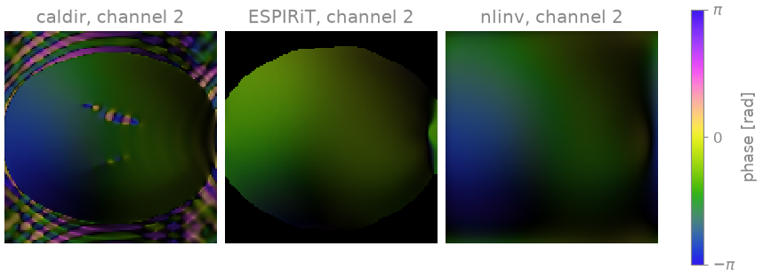
Here is channel 2 from each: brightness is the magnitude and colour the phase. The phase of a set of maps is only defined up to a phase common to all channels, which each estimator fixes its own way; that common phase passes into the phase of the image and leaves its magnitude alone. Up to it, the three agree inside the object. Outside it the data say nothing about a sensitivity, and the estimators return different values there: caldir divides noise by noise and returns an arbitrary value of unit magnitude, ESPIRiT sets the maps to zero, and nlinv continues the smooth function its regularization favours.

SENSE and map quality

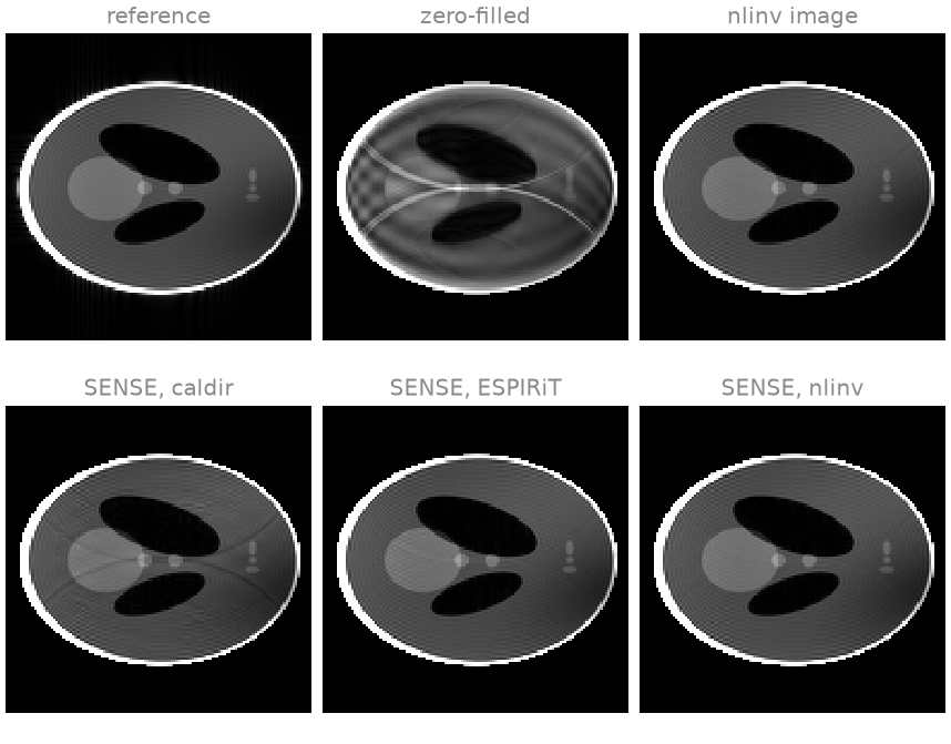
Now you give each set to bartorch.apps.pics() with the same Tikhonov weight and the same number of conjugate-gradient iterations, so the only thing that differs is the maps. The image nlinv returned with its maps is a fourth estimate.

reconstructions = {
    name: apps.pics(measured, maps, l2=0.001, maxiter=40)
    for name, maps in (
        ("caldir", direct),
        ("ESPIRiT", espirit),
        ("nlinv", nonlinear),
    )
}

for name, estimate in reconstructions.items():
    print(f"{name:>12}  NRMSE {error(estimate):.3f}")
print(f"{'nlinv image':>12}  NRMSE {error(joint):.3f}")

• 
• 

     caldir  NRMSE 0.025
    ESPIRiT  NRMSE 0.015
      nlinv  NRMSE 0.012
nlinv image  NRMSE 0.011

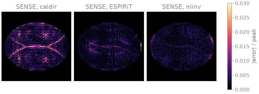
All three sets of maps unfold the three copies, and so does nlinv on its own. The error maps, at 3 % of the image peak, show what is left. The direct estimate leaves a faint residual fold at the edges of the phantom, where its low-resolution maps are least accurate; ESPIRiT and nonlinear inversion leave mostly noise.

ACS size

Now you keep only eight central lines. ESPIRiT’s kernel is six samples wide by default, so eight lines leave it three positions along the phase-encoding axis, and its calibration matrix has too few rows. caldir still runs, on an image of eight lines’ resolution. nlinv uses every acquired sample, so the ACS region affects it only through its first Gauss-Newton steps.

scarce = acquire(8)

espirit = bt.ecalib(scarce, maps=1, calib_size=8, crop=0.8)
covered = float((espirit.abs() > 0).float().mean())
print(f"ESPIRiT: {covered:.0%} of voxels with a sensitivity")

direct = bt.caldir(scarce, 8)
joint, estimated = bt.nlinv(scarce, maxiter=12, return_sensitivities=True)
rss_maps = bartorch.rss(estimated, axes=(0,), keepdim=True)
nonlinear = estimated / rss_maps.abs().clamp(min=1e-6)

scarce_reconstructions = {
    "caldir": apps.pics(scarce, direct, l2=0.001, maxiter=40),
    "nlinv": apps.pics(scarce, nonlinear, l2=0.001, maxiter=40),
    "nlinv image": joint,
}
for name, estimate in scarce_reconstructions.items():
    print(f"{name:>12}  NRMSE {error(estimate):.3f}")

• 
• 

ESPIRiT: 0% of voxels with a sensitivity
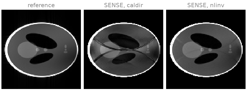
      caldir  NRMSE 0.173
       nlinv  NRMSE 0.040
 nlinv image  NRMSE 0.033

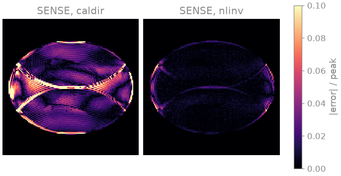
ESPIRiT returns maps that are zero in every voxel, which no reconstruction can use. With the direct estimate you see residual aliasing: maps at the resolution of eight lines do not follow the coil profiles closely enough to unfold three copies, and the folded edges of the skull reappear inside the phantom (the error maps are now at 10 % of the peak). The maps from nonlinear inversion still unfold the image, because they are fitted to all the acquired samples. The same estimator works on non-Cartesian data, where there is no Cartesian ACS region at all, as bartorch.tools.ncalib(), which you use in lesson 8 (8. Radial SENSE).

These errors are for one phantom, one noise level and one sampling pattern, and they depend on how each reconstruction is regularized; they do not rank the estimators in general.

Exercise: ACS size

Between eight and 24 lines the outcome changes. Sweep the size of the ACS region for the two estimators that use only the ACS block, and compare how their errors depend on it:

sizes = (12, 16, 24, 32)
scores = {"caldir": [], "ESPIRiT": []}
for lines in sizes:
    data = acquire(lines)
    maps = {
        "caldir": bt.caldir(data, lines),
        "ESPIRiT": bt.ecalib(data, maps=1, calib_size=lines, crop=0.8),
    }
    for name, estimate in maps.items():
        image = apps.pics(data, estimate, l2=0.001, maxiter=40)
        scores[name].append(error(image))

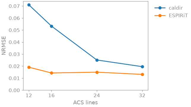
12 lines: caldir 0.071, ESPIRiT 0.019
16 lines: caldir 0.053, ESPIRiT 0.014
24 lines: caldir 0.025, ESPIRiT 0.015
32 lines: caldir 0.020, ESPIRiT 0.013

The ESPIRiT error is close to its 24-line value from twelve lines on: once the kernel has enough positions in the ACS region, more lines add little. The caldir error keeps falling as the region grows, because its maps are only as sharp as the ACS image they are computed from, and it stays above ESPIRiT’s at every size here. Try crop values between 0.5 and 0.95 for ESPIRiT, or another maxiter for nlinv at eight lines, and see how the errors move.

As a spec

What this lesson built, stated the way you would ask an agent for it:

With bartorch, simulate 8-channel analytical k-space of a 128x128
Shepp-Logan phantom (bt.phantom(coils=8, kspace=True)) with noise of
variance 2. Keep every third phase encode plus a fully sampled central
ACS block. Estimate sensitivities three ways: bt.caldir, bt.ecalib
(one map, crop 0.8) and bt.nlinv (12 Gauss-Newton steps, maps divided
by their root sum of squares). Reconstruct with apps.pics (l2=0.001,
40 CG iterations) using each set, and report the NRMSE of the magnitude
inside the phantom against the noise-free RSS image, after a global
scale. Repeat with 24 and with 8 ACS lines.

References

[1]

Pruessmann KP, Weiger M, Scheidegger MB, Boesiger P. SENSE: sensitivity encoding for fast MRI. Magn Reson Med 42(5):952-962 (1999). https://doi.org/10.1002/(SICI)1522-2594(199911)42:5%3C952::AID-MRM16%3E3.0.CO;2-S

[2]

Uecker M, Lai P, Murphy MJ, Virtue P, Elad M, Pauly JM, Vasanawala SS, Lustig M. ESPIRiT – an eigenvalue approach to autocalibrating parallel MRI: where SENSE meets GRAPPA. Magn Reson Med 71(3):990-1001 (2014). https://doi.org/10.1002/mrm.24751

[3]

Uecker M, Hohage T, Block KT, Frahm J. Image reconstruction by regularized nonlinear inversion – joint estimation of coil sensitivities and image content. Magn Reson Med 60(3):674-682 (2008). https://doi.org/10.1002/mrm.21691