tools.nlinv

bartorch.tools.nlinv()

Image and coil sensitivities estimated jointly by nonlinear inversion.

Parameters:

• kspace (torch.Tensor) – Undersampled k-space, (..., coils, z, y, x).

• maxiter (int, default=None) – Number of Gauss-Newton steps (-i); BART’s default is 8.

• maps (int, default=None) – Number of sets of sensitivities, ENLIVE (-m).

• traj (torch.Tensor, default=None) – Non-Cartesian trajectory (..., samples, 3) in grid units (-t).

• pattern (torch.Tensor, default=None) – Sampling pattern (-p).

• basis (torch.Tensor, default=None) – Temporal subspace basis (-B).

• initial (torch.Tensor, default=None) – Initial image and sensitivities (-I).

• alpha (float, default=None) – a of the Sobolev weighting (1 + a |k|^2)^(-b/2) of the sensitivities (-a). The regularization weight of the first Gauss-Newton step is nlinv --alpha, passed through **extra.

• real (bool, default=False) – Constrain the image to be real (-c).

• normalize (bool, default=True) – Multiply the image by the root sum of squares of the sensitivities over the coils (see Notes); False is BART’s -N.

• return_sensitivities (bool, default=False) – Also return the sensitivities, BART’s optional second output.

• **extra – Further BART nlinv options, by name. s, the axes the sensitivities are constant along, takes axes of kspace.

Returns:

The image, without the coil axis and with the sets of maps combined, and the sensitivities when asked for.

Return type:

torch.Tensor or tuple of torch.Tensor

Notes

With normalize=True and one set of sensitivities, the returned image is \(\rho \sqrt{\sum_c |s_c|^2}\): the magnitude of the coil images \(\rho s_c\) combined by root sum of squares, with the phase of \(\rho\). With several sets combined it is \(\sqrt{\sum_c |\sum_m \rho_m s_{m,c}|^2}\), which is real.

Examples using nlinv

3. Coil sensitivities

3. Coil sensitivities

4. Joint reconstruction of image and sensitivity maps

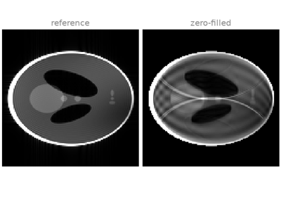
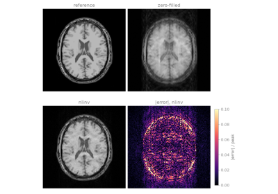
4. Joint reconstruction of image and sensitivity maps