nlop.IRGNM#

class bartorch.nlop.IRGNM#

Bases:

Iteratively regularized Gauss-Newton solver for F(x) = y.

Each step linearizes F at the current iterate and solves

min_u ||DF u - r||^2 + alpha ||u||^2 + R(u)

for the residual r carried to the linearization; alpha is then decayed towards alpha_min by redu. R is the regularization of the inner solver, and absent for conjugate gradients. The solver loops IRGNMBlock, which documents the two forms.

Parameters:

iterations (int, default=8) – Gauss-Newton steps.
alpha (float, default=1.0) – Tikhonov weight of the first step.
alpha_min (float, default=0.0) – Limit the weight decays towards.
alpha_min0 (float, default=0.0) – Lower bound on the decayed weight; used only with inner.
redu (float, default=2.0) – Decay factor of the weight per step.
cg_maxiter (int, default=30) – Conjugate-gradient iterations per step without inner.
cg_tol (float, default=0.0) – Conjugate-gradient tolerance per step without inner.
inner (solver, default=None) – Configured solver from bartorch.optim for the linearized problem, whose regularizers are R. None solves it by conjugate gradients inside the library, as nlinv does.
fuse (bool, default=True) – Apply the encoding of a coil model as its normal operator; see IRGNMBlock.plan().

Notes

The two forms agree in exact arithmetic but not to the bit: without inner the result matches BART’s iter4_irgnm, and with inner=optim.CG() it matches iter4_irgnm2.

Examples

Plain, which is nlinv:

>>> nlop.IRGNM(iterations=8)(kspace, F, x0=start)

The same method with the linearized problem written out here, which is iter4_irgnm2 to the bit:

>>> nlop.IRGNM(iterations=8, inner=optim.CG())(kspace, F, x0=start)

Wavelet-regularized:

>>> nlop.IRGNM(inner=optim.FISTA(priors.Wavelet((-1, -2), 0.001), maxiter=30))(
...     kspace, F, x0=start
... )

Several terms at once, which is ADMM’s job:

>>> nlop.IRGNM(
...     inner=optim.ADMM(
...         [priors.Wavelet((-1, -2), 0.001), priors.TotalVariation((-1, -2), 0.01)]
...     )
... )(kspace, F, x0=start)

__call__()#

Solve F(x) = y.

Parameters:

y (torch.Tensor) – Data of F.oshape, with an optional leading batch axis.
F (NonlinearOperator or LinearOperator) – Forward model; a linear one is converted with to_nonlinear().
x0 (torch.Tensor or tuple of torch.Tensor, default=None) – Start; see IRGNMBlock.start().
xref (torch.Tensor or tuple of torch.Tensor, default=None) – Regularization centre; None regularizes towards zero, as BART does.

Returns:

Complex64 solution, one tensor per input of F.

Return type:

torch.Tensor or tuple of torch.Tensor

Examples using `IRGNM`#

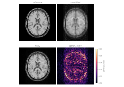
4. Joint reconstruction of image and sensitivity maps

9. Nonlinear inversion for T2 mapping

nlop.IRGNM

Contents

nlop.IRGNM#

Examples using IRGNM#

Examples using `IRGNM`#